Demand Forecast#
In today’s fast-moving markets, anticipating demand with precision is critical to making confident, informed decisions. ConverSight’s Demand Forecast empowers business users to plan proactively by transforming historical data into actionable demand insights—without needing technical expertise.
Built with flexibility and control at its core, this feature guides users through a structured forecasting journey. From configuring scenario preferences and selecting the right datasets to reviewing and adjusting projections, every step is designed for usability and impact. Users can create new forecasting scenarios, apply classification logic, fine-tune values and publish forecasts organization-wide—all within an intuitive interface. Whether you’re refining forecasts manually or using AI Demand Forecast models, the platform gives you complete visibility and control.
This documentation walks you through each section of the application, providing step-by-step instructions to help you confidently create, manage and publish forecasts that drive results.
Accessing Demand Forecast#
The Demand Forecast application can be accessed by navigating to the Launchpad tab and selecting the Demand Forecast app.
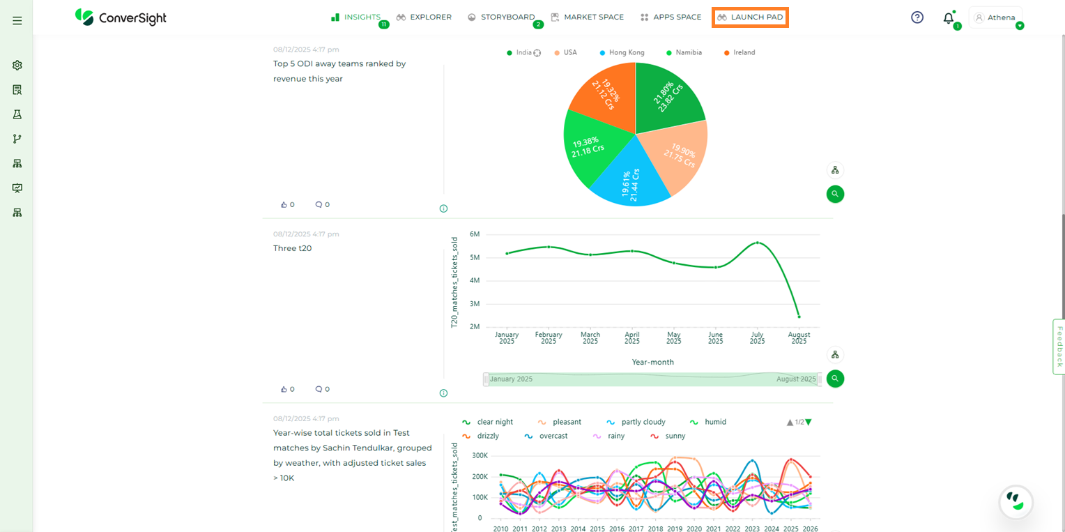
Launchpad Tab#
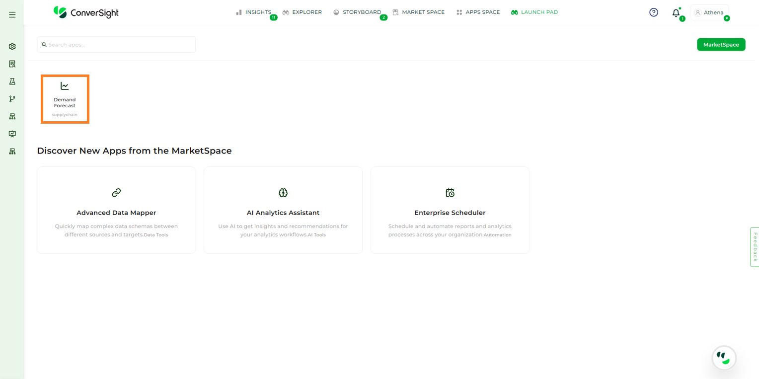
Demand Forecast App#
Forecast Tabs Overview#
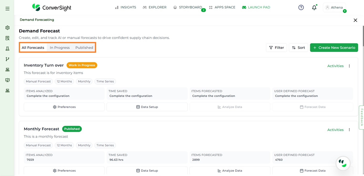
The Demand Forecast page includes three tabs that provide users with access to different forecast statuses:
All Forecasts – Displays all forecasts, including created, in-progress, and published ones.
In Progress – Displays only the forecasts that are currently in progress.
Published – Displays only the forecasts that have been published.
Demand Forecast Overview#
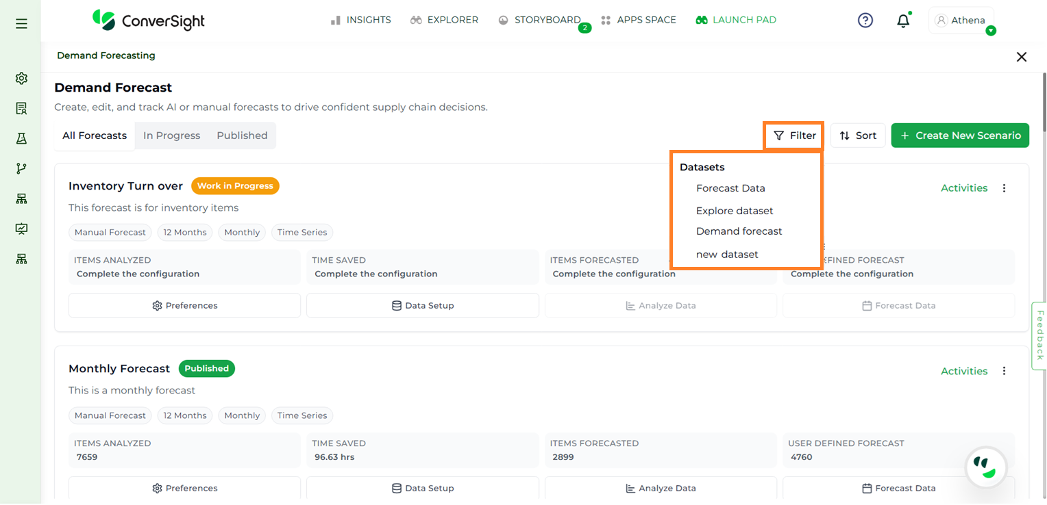
Filters#
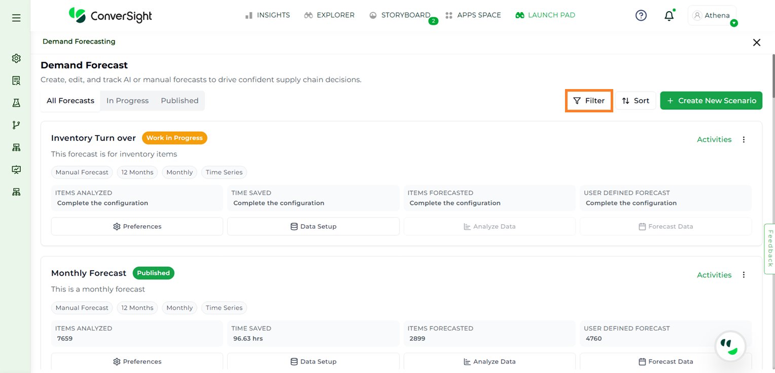
To streamline the view, users can filter forecasts based on Forecast Types and Datasets by selecting the Filter button available on the Demand Forecast page.
Filters#
Under Forecast Type, the following options are available:
All Forecast Types – Displays all forecasts in the system, regardless of how they were created.
AI Model Forecast – Displays only those forecasts that were generated using AI models.
Manual Forecast – Displays only the forecasts that were manually created by users.
Filters#
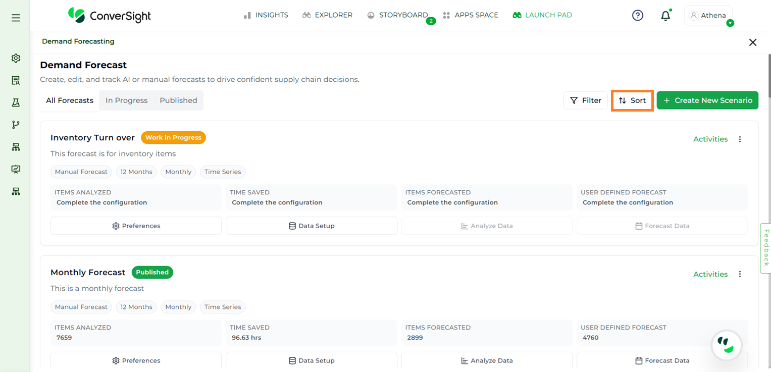
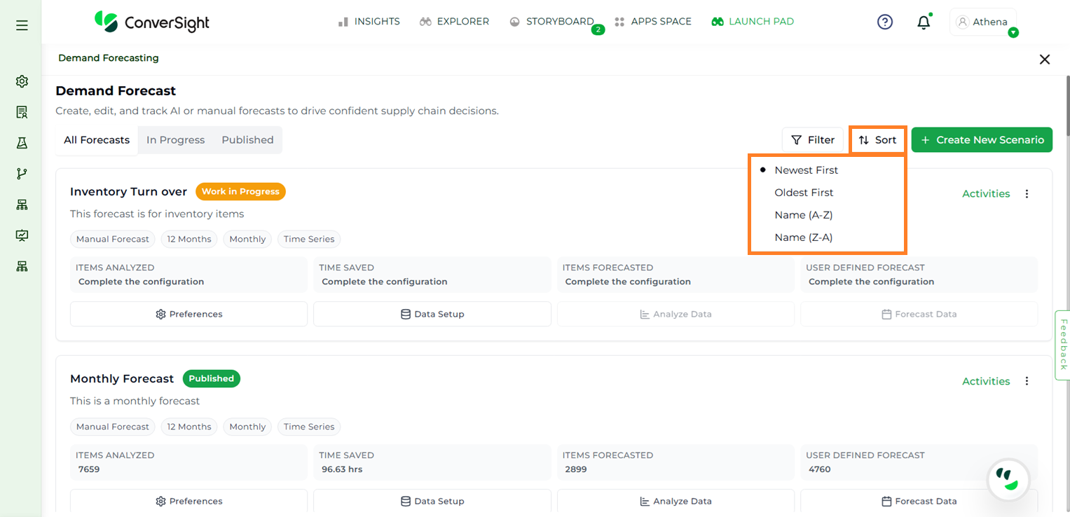
Sort#
Users can organize the list of forecasts using the Sort feature, which allows sorting based on specific preferences. Forecasts can be sorted in ascending or descending order, as well as by newest first or oldest first, depending on user requirements.
Sort#
Sort#
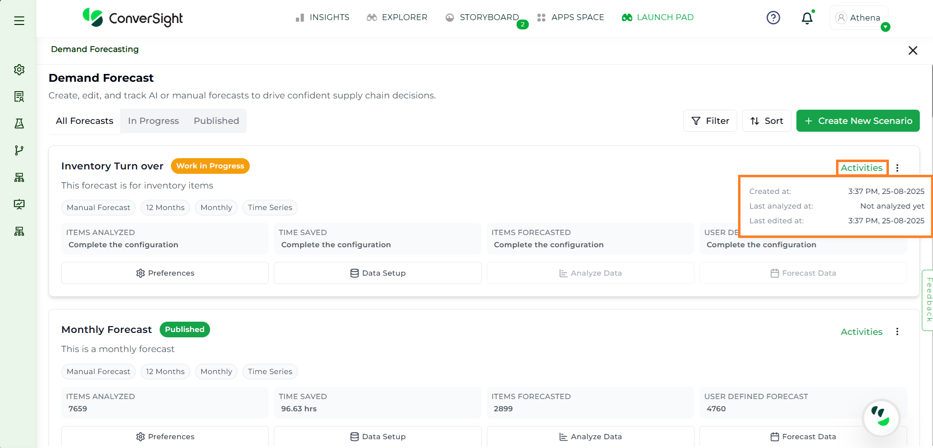
Activities#
The Activities section provides a summary of key timestamps, including when the forecast was created, last analyzed and last edited.
Activities#
Clicking the three-dot menu opens a dropdown with two options: Edit and Delete.
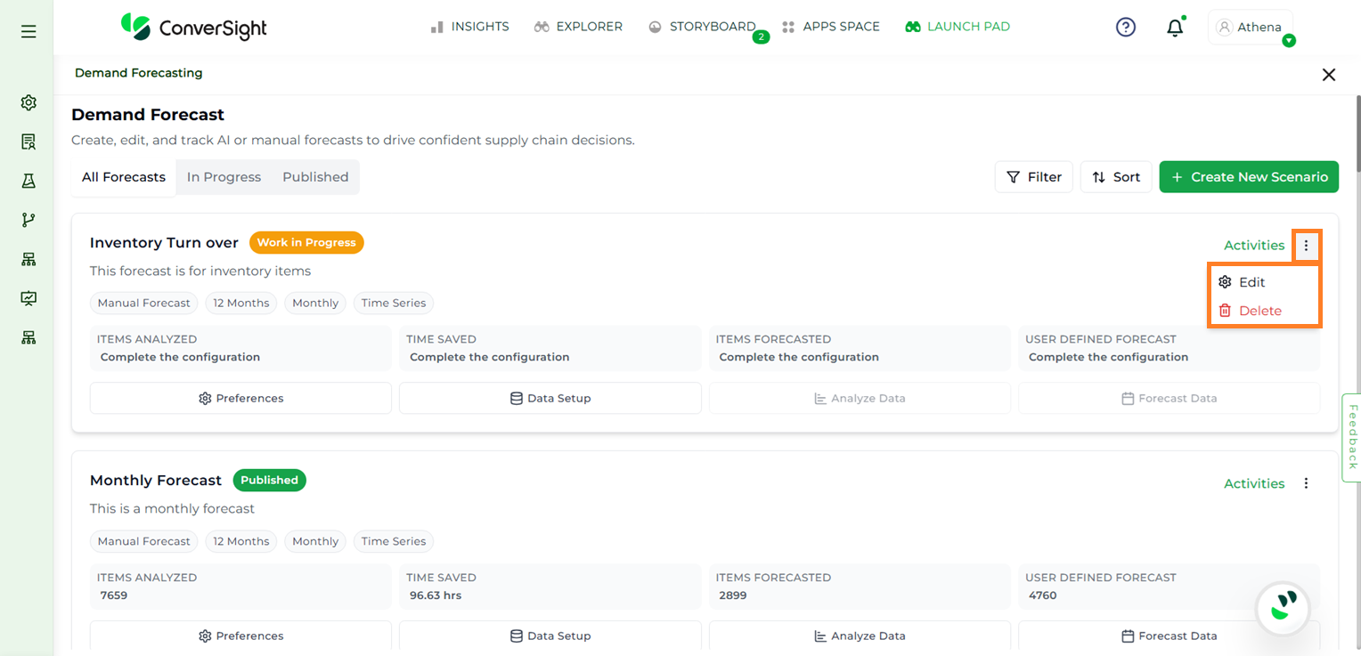
Activity#
Selecting Edit allows users to modify the existing forecast.

Edit#
Selecting Delete prompts a confirmation popup. Click Delete in the popup to permanently remove the forecast.
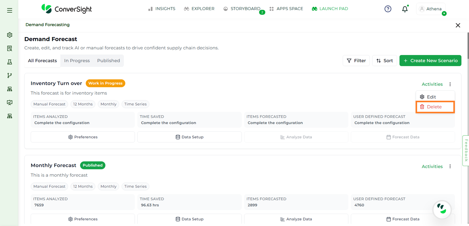
Delete#
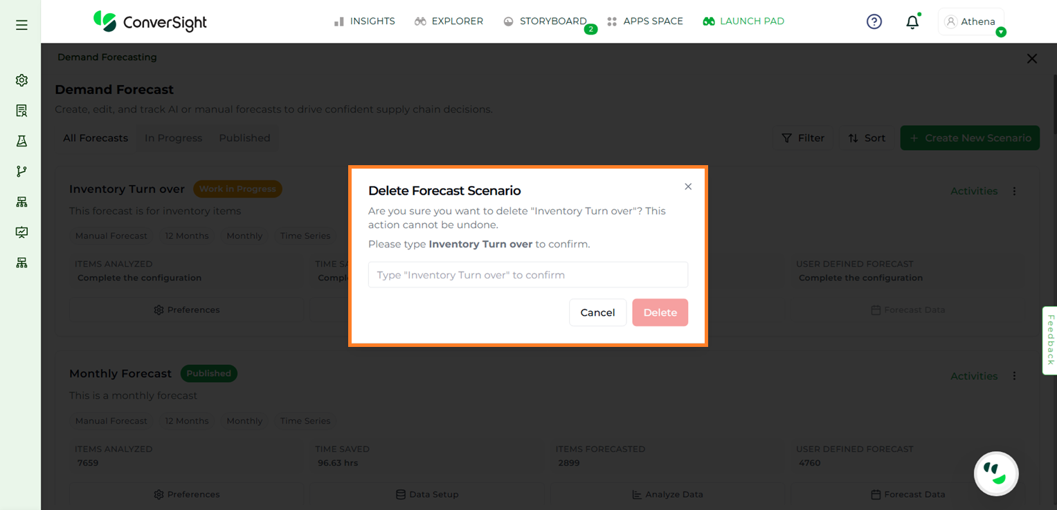
Delete#
Users can duplicate an existing configuration by selecting the Clone option. After cloning, they can rename the configuration and save it as a new one.
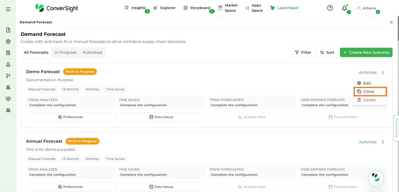
Clone#
Create New Scenario#
To create a new forecast, users can click the + Create New Scenario button on the Demand Forecast page. Before generating the forecast, the application analyzes the input data. During scenario creation, it gathers user preferences and configures the necessary data setup to enable accurate forecasting.
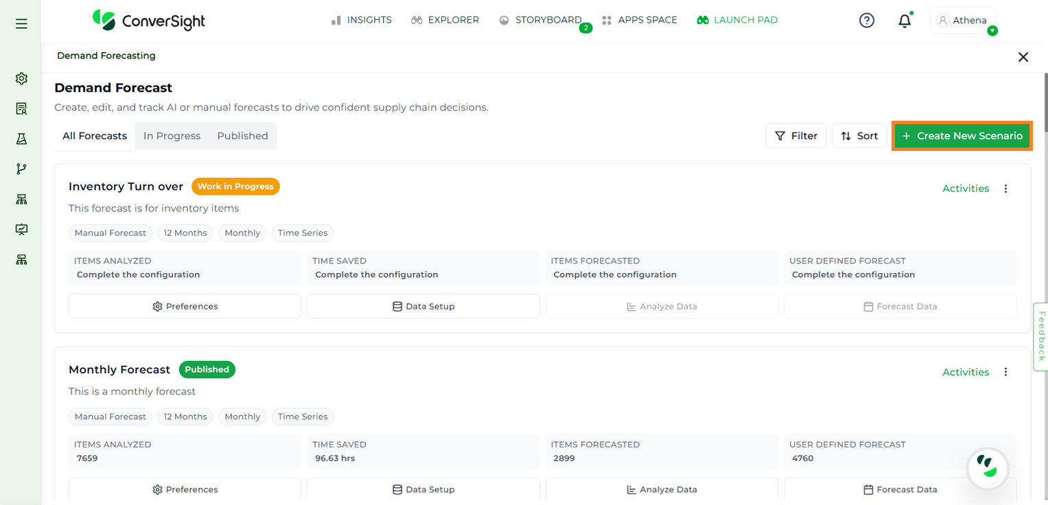
Create New Scenario#
The forecast creation process consists of four key stages:
Preferences
Data
Analyze Data
Forecast Data
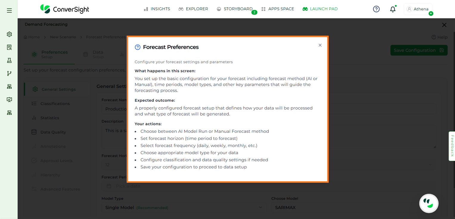
NOTE
The Help feature available on each page provides users with a guided overview of the screen. It explains the purpose of the page, the expected outcomes, and the actions users can take.
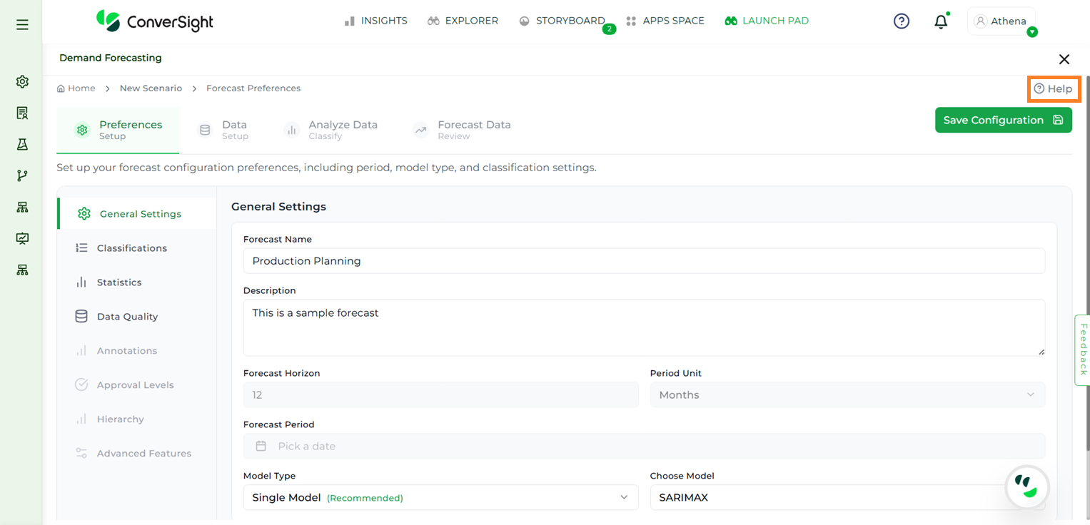
Demand Forecast Help#
Demand Forecast#
Preferences#
The Preferences stage defines the foundational settings that guide how a forecast is generated and interpreted. It ensures the forecast aligns with business goals by setting horizons and units, standardizes methodology through classifications and statistical parameters, and improves reliability by addressing data quality issues such as outliers or missing values. By configuring these options up front, users create a structured base that makes the subsequent stages—Data Setup, Analyze Data, and Forecast Data—more accurate, consistent, and relevant to decision-making.
The Preferences stage includes four steps to configure the foundational settings for a new forecast:
General Settings
Classifications
Statistics
Data Quality
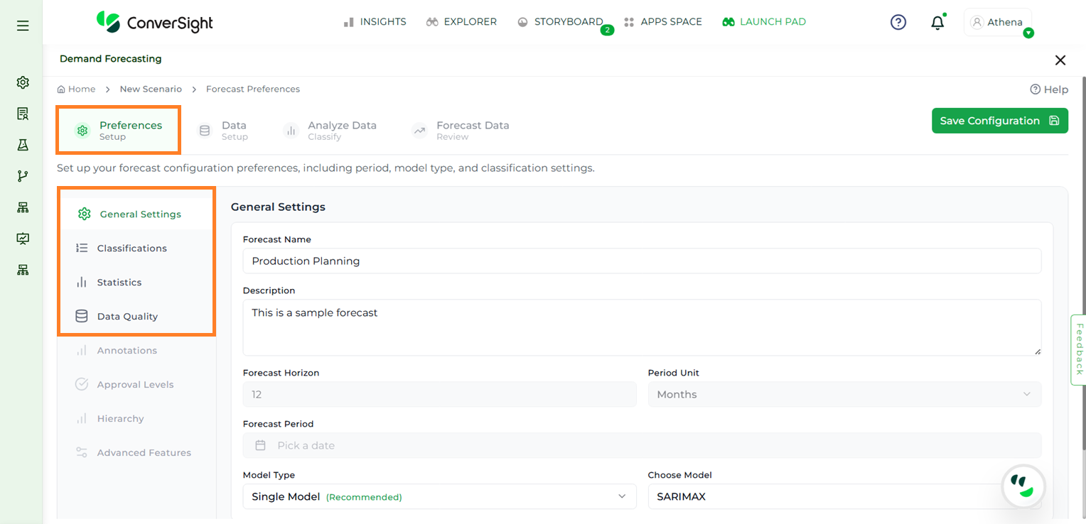
Preferences#
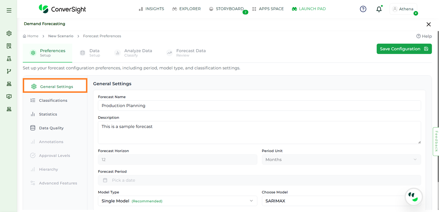
General Settings#
In this step, users are required to provide essential details required to setup a new configuration.
Field |
Description |
|---|---|
Forecast Name |
Users must provide a unique name for the forecast scenario, which will serve as the reference table name for the forecast output. The Forecast Name field supports a maximum of 20 characters. |
Description |
Provide a clear and meaningful description for your configuration to help identify its purpose and facilitate future reference. |
Forecast Horizon |
Specify the number of months to forecast. |
Period Unit |
Select the forecast granularity such as Monthly, Daily, or Yearly. |
Forecast Period |
Users can select the desired forecast period while creating a new forecast configuration. This option is available only at the time of creation and will be disabled when editing an existing configuration. |
Model Type |
Users can choose the type of forecasting model required. The available options are Single Model and Multi Model. Multi Model is available only for premium users. |
Choose Model |
Choose the forecasting model to apply. At present, SARIMAX (Seasonal Autoregressive Integrated Moving Average with exogenous factors) is the default and the only available option. |
General Settings#
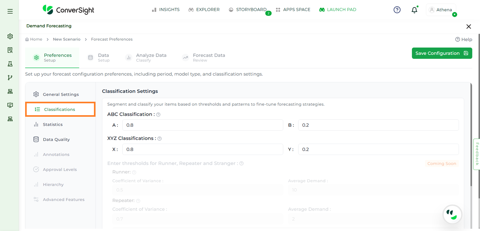
Classifications#
In the Classifications step, users can segment and categorize items based on specific thresholds and demand patterns to refine their forecasting strategies. The app automatically categorizes items into three classes—A, B, or C—based on how much each item contributes to a specific metric (such as revenue, sales volume, or demand), when all items are considered together.
The available classification methods include:
ABC Classification
XYZ Classification
ABC Classification#
ABC classification groups items based on how much they contribute to a selected metric, such as sales or revenue.
A-class items are the top contributors and together make up approximately the first 80 percent of the total value.
B-class items contribute the next 20 percent, bringing the total to around 100 percent.
C-class items include any remaining items beyond the A and B groups.
NOTE
The HelpThese classifications are based on the ranking of items by their contribution, not on the total number of items. In most cases, items fall into A and B categories, and C-class may not always include additional items.
XYZ Classification#
XYZ classification helps group items based on how much their demand changes over time. This is measured using a statistical value called the coefficient of variation.
X-class items have low demand variation, meaning their demand is stable and predictable.
Y-class items show moderate changes in demand.
Z-class items have high demand variation, making them more unpredictable.
The app uses predefined threshold values to automatically assign items to these categories. This helps improve the accuracy of forecasts by identifying which items are stable and which are more variable. Users can define thresholds for each classification as needed. Additional options such as thresholds for runner, repeater, and stranger categories, as well as classifications based on recency, sparsity, and others, are currently unavailable and will be introduced in future updates.
Classifications#
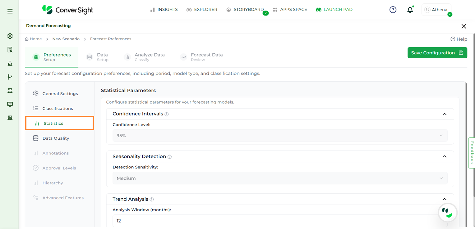
Statistics#
The Statistics step allows users to fine-tune their forecasting models by adjusting key parameters:
Confidence Level: The confidence interval indicates the level of certainty in the forecast results. By default, the confidence level is set to 95%, meaning the actual demand is expected to fall within the forecasted range 95% of the time. This helps assess the reliability of the forecast.
Seasonality Detection: Seasonality detection identifies recurring patterns in the data, such as monthly spikes or seasonal dips. A Medium sensitivity level is applied by default to maintain a balanced approach—capturing meaningful trends without reacting to short-term noise.
Trend Analysis: Trend analysis reveals the long-term direction of demand, such as whether it is increasing, decreasing, or stable. This is done using linear regression applied over a default time window of 12 months. The analysis window can be adjusted to define how many months should be included in the trend evaluation.
Statistics#
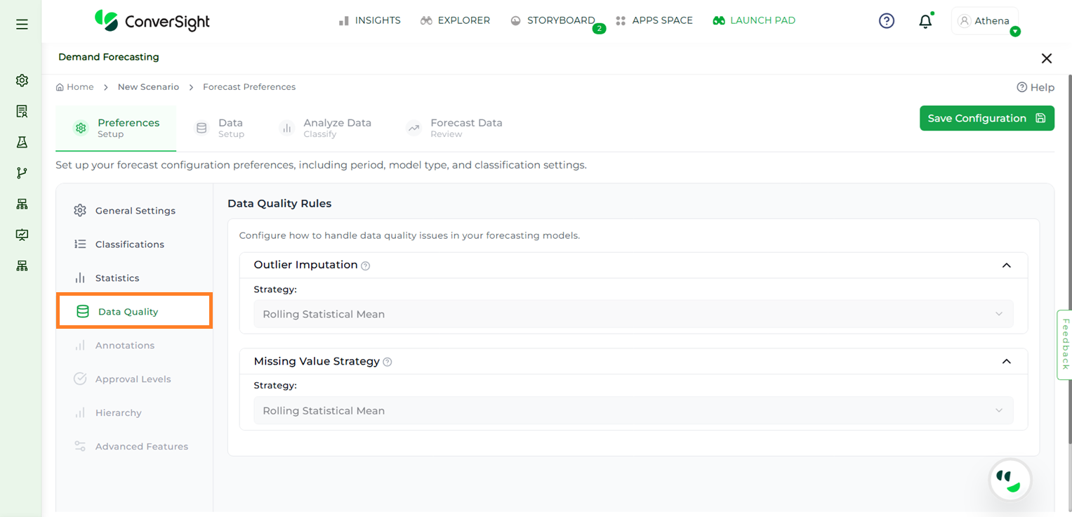
Data Quality#
The Data Quality step enables users to manually configure how data issues should be addressed. Users can choose to enable or disable the following rules based on their specific forecasting requirements:
Outlier Imputation – Allows users to handle abnormal or extreme values in the dataset that could impact forecast accuracy.
Missing Value Strategy - Enables users to define the missing entries in the dataset.
These options are enabled by default. The default strategy applied is Rolling Statistical Mean, which uses a moving average technique to fill or adjust data values, ensuring the dataset is prepared for consistent and accurate forecasting.
Data Quality#
After completing the above steps, users must click the Save Configuration button. This action will navigate them to the Data Setup page.
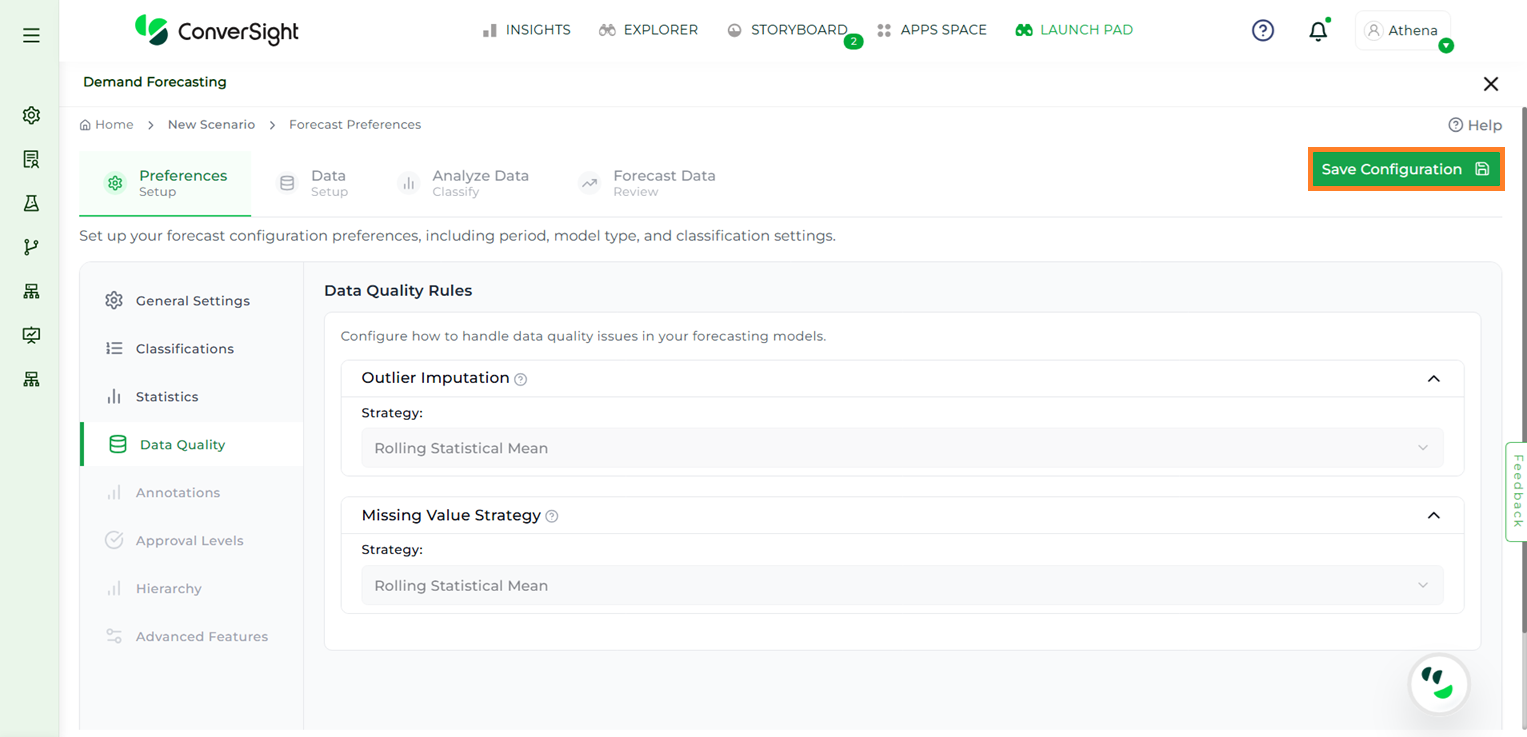
Save Configurations#
Data#
The Data stage requires users to select the dataset and specific columns that will be used to generate the forecast. To meet the minimum data validation criteria, users must select one dimension column, one metric column and one date column.
NOTE
Only Input v2 datasets are supported for creating forecast configurations.
To begin:
Step 1: Click the Explore button.
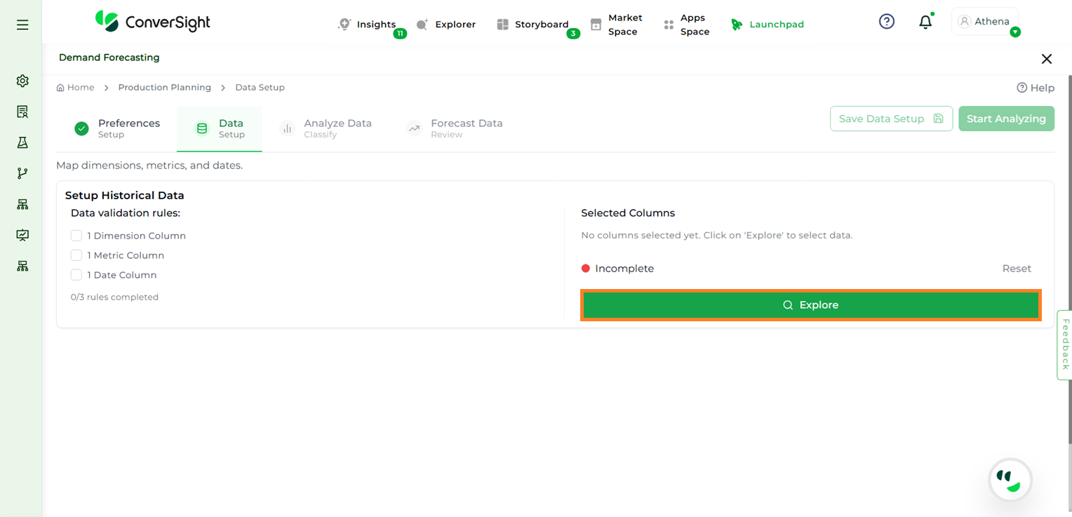
Explore#
Step 2: From the dataset dropdown, choose the desired dataset.
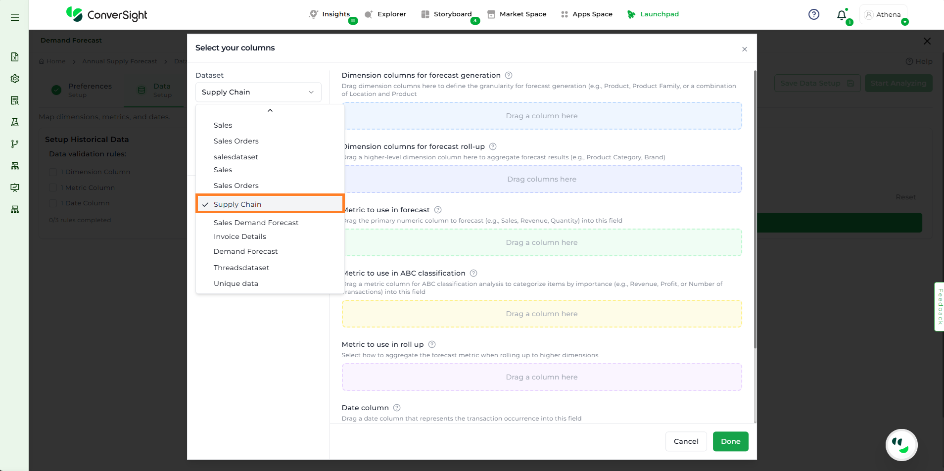
Dataset Selection#
Step 3: Select the relevant Subject Area.
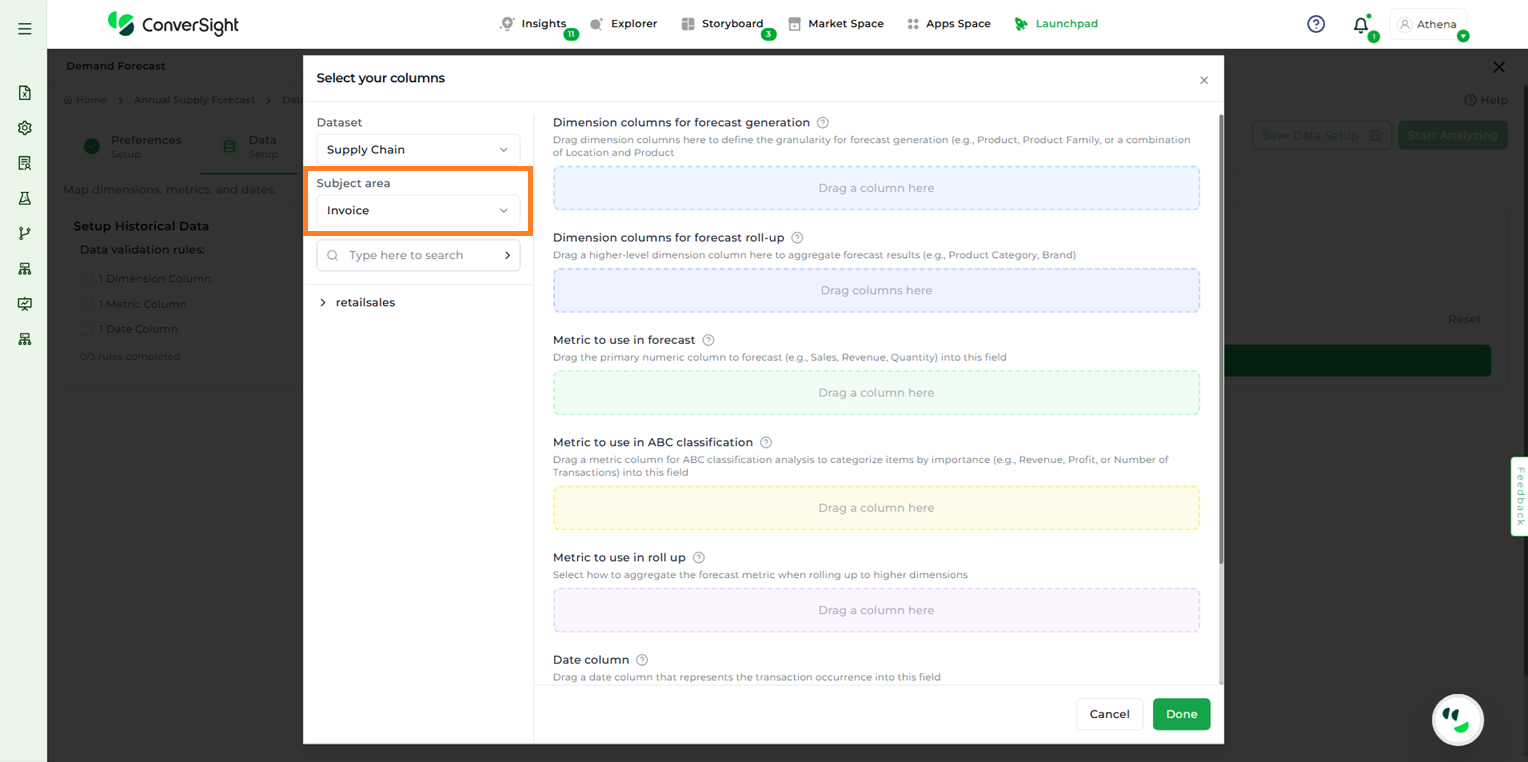
Subject Area#
Step 4: Drag and drop the appropriate dimension, metric and date columns into the designated sections.
The Available column Sections:
Dimension columns for forecast generation: Used to generate forecasts at the lowest level (e.g., forecast demand for each SKU).
Dimension columns for forecast roll-up (optional): Groups forecasts into higher-level summaries (e.g., SKU → Category → Region).
Metric to use in forecast: The numeric value the model will use to generate demand predictions.
Metric to use in ABC classification (optional): Used for classifying items into A (high value), B (medium value), or C (low value) categories, which helps in prioritization.
Metric to use in roll-up: Defines which metric should be summed when aggregating forecasts from lower to higher levels.
Date Column: Ensures the forecast is tied to a time dimension (day, week, month).
Filter Data (optional): Optional filters to limit the dataset (e.g., Region = North America, Product Type = Electronics).
Step 5: Once the selections are complete, click Done.
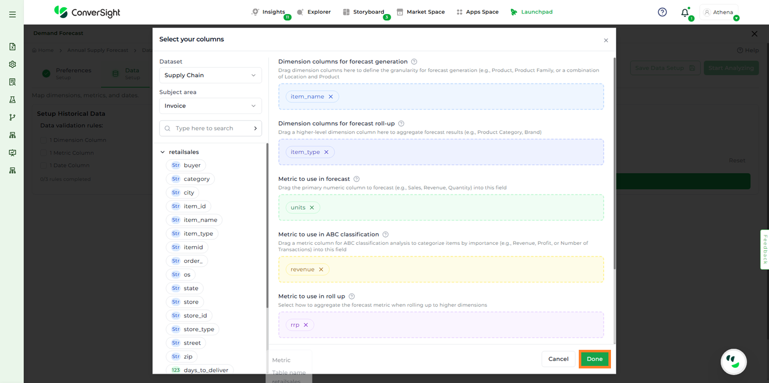
Choosing columns#
NOTE
If the selected columns meet the validation rules, a checkmark will appear next to each criterion, confirming the requirement has been satisfied.
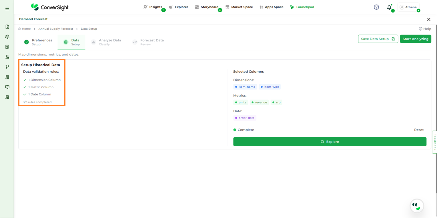
Rules Validation#
The Selected Columns section will display the currently chosen dimension, metric and date columns. If changes are needed, click Reset to clear the selections, then click Explore again to reselect the desired columns.
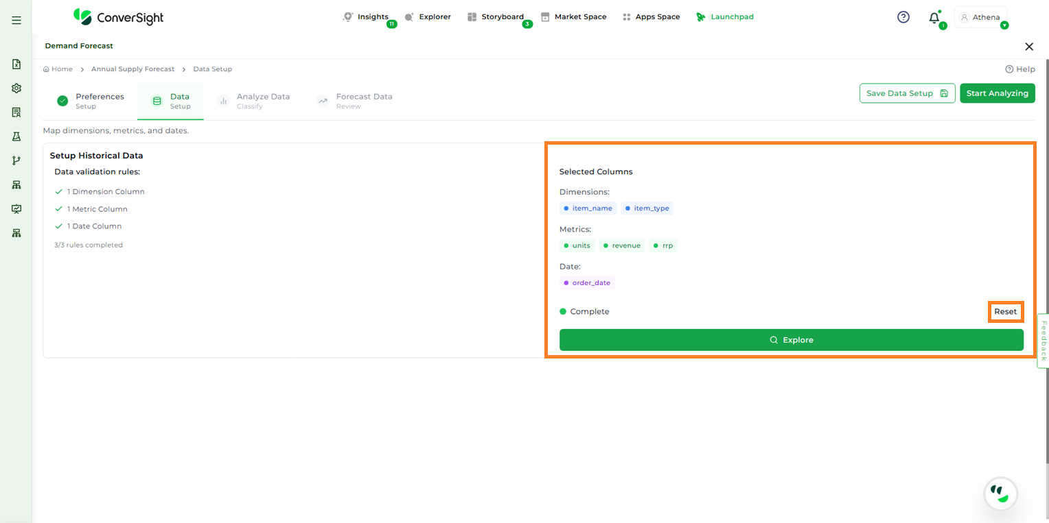
Columns Reset#
After completing the Data Setup, users have two options:
Click Save Data Setup to save progress and return later to continue the forecasting process.
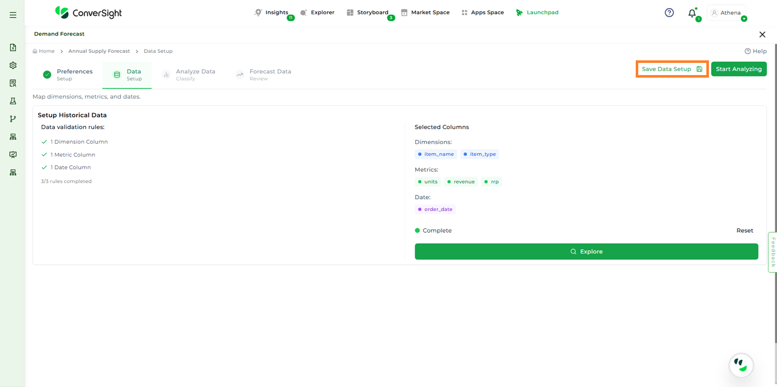
Save Data Setup#
Click Start Analyzing to proceed to the next step. Choosing this option will open a windows asking whether to Save and Start Analysis or Cancel. Click on the Save and Start Analysis button to go to the Analyze Data stage.
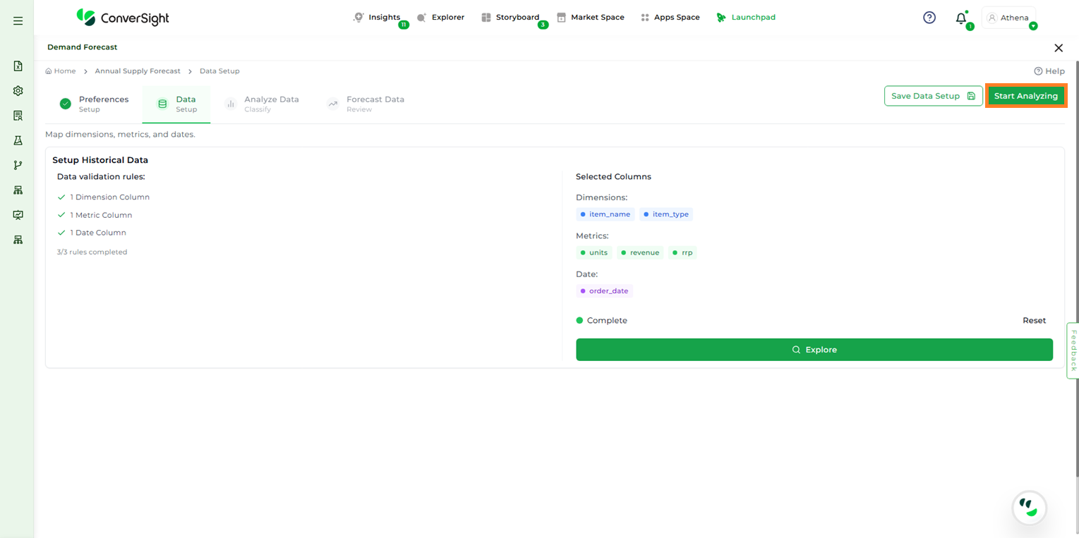
Start Analysis#
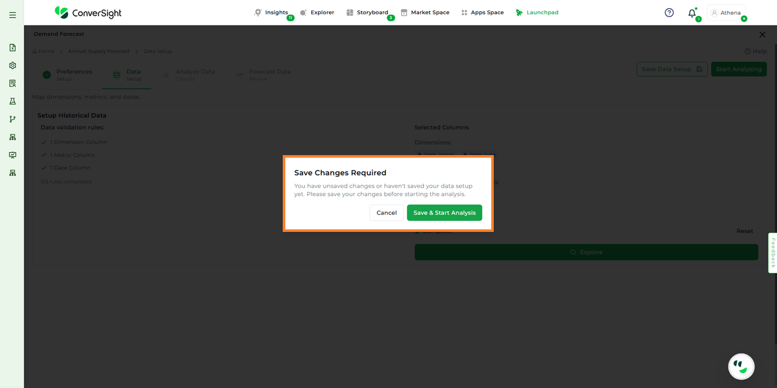
Start Analysis#
Analyze Data#
In the Analyze Data step, users can thoroughly review and prepare their data before running the forecast. This stage provides the flexibility to classify data, select specific SKUs for forecasting and either input forecast values manually or reuse values from previous forecasts.
To streamline navigation, users can search for specific dimension columns using the Search bar.
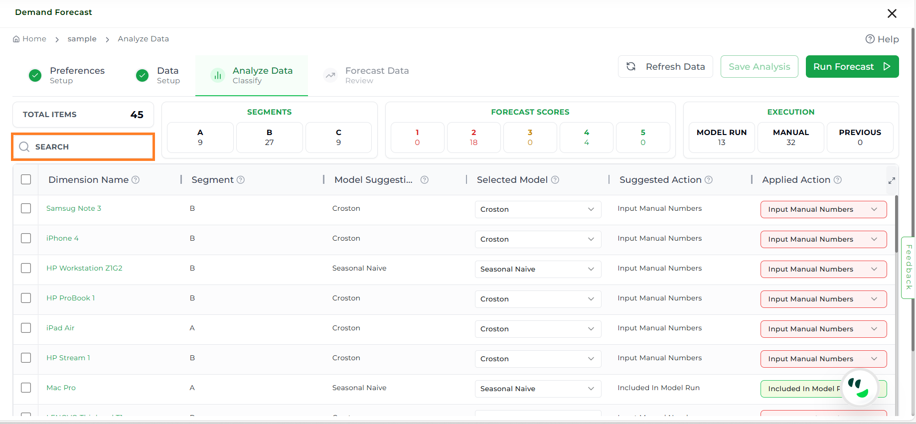
Search Dimension#
The Total Items section displays the number of items after filtering. Users can further refine the view by selecting a specific segment to see items related only to that segment.
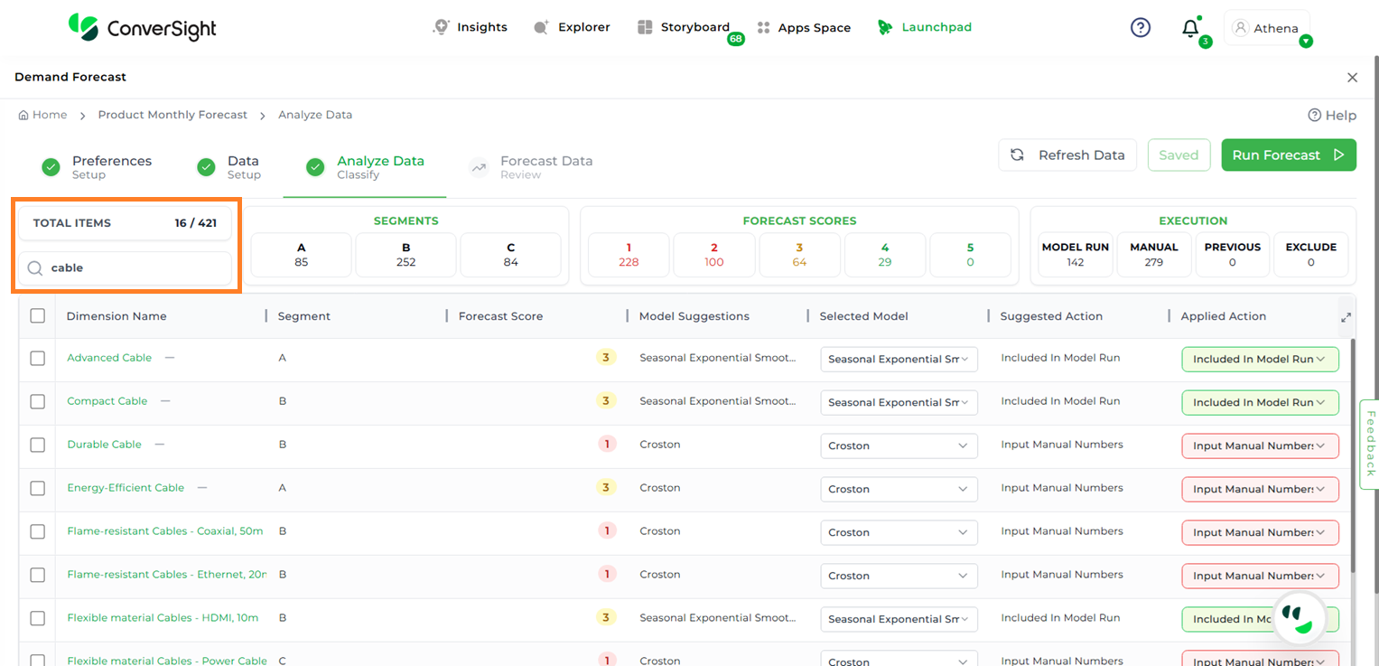
Search Dimension#
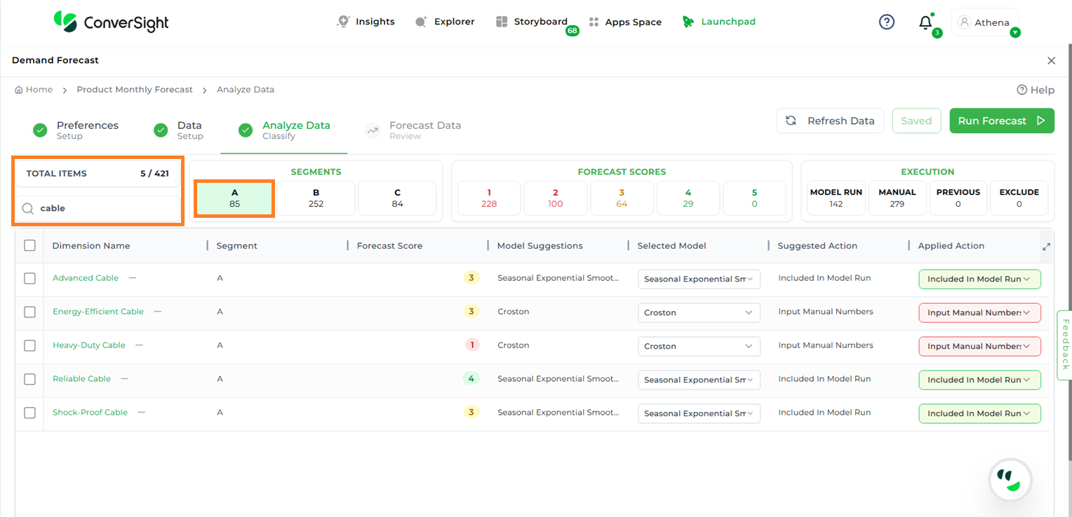
Search Dimension By Segment#
If there are updates to the dataset, clicking the Refresh Data button will reload the most recent data.
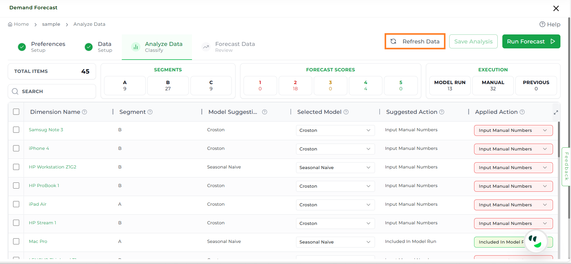
Refresh Data#
The Analyze Data page also displays key summary metrics, including:
Total SKUs: The total number of SKUs available for forecasting
Segments: Groups of data based on dimension columns (e.g., forecasts per SKU).
Segment A: Represents high-priority or high-value items, typically the top 10–20% of SKUs.
Segment B: Indicates medium-priority or moderate-value items, generally the next 20–30% after Segment A.
Segment C: Covers low-priority or low-value items, usually the bottom 50–70% of SKUs.
Forecastability Score (1–5) – Indicates how predictable the dataset is.
1 = Low predictability (erratic data).
5 = High predictability (stable patterns).
Execution Category: Defines how forecasts will be executed:
Model Run: Displays the forecasting model applied to the selected SKUs.
Manual: Indicates the number of SKUs with manually entered forecast values.
Previous Forecast: Represents the number of SKUs where forecast inputs were taken from previously generated forecasts.
Exclude from Forecast: Excludes the selected items from the forecast.
Detailed Data View#
Users are presented with a comprehensive table view of their dataset, where each row is analyzed and classified using various statistical and forecasting techniques.
The table includes the following columns for in-depth analysis:
Column Name |
Description |
|---|---|
Dimension Name |
This is the name of the item or segment being forecasted. |
Segment |
Helps group items into priority segments (like A, B, or C) so customers can focus efforts on what matters most. |
Forecast Score |
Indicates the level of forecastability of the item or segment. |
Model Suggestion |
AI recommends the best-fit models based on data patterns like trend, seasonality, and variability. Each comes with a short definition and ideal use case to guide selection. |
Selected Model |
The model chosen to generate the final forecast. Athena AI auto-selects the best option, but users can override if needed. |
Suggested Action |
The Suggested Action column tells you what action to take such as including in the model run, excluding, or using the previous forecast based on the latest data behaviour. The suggested action is determined dynamically each time you run the analysis, according to predefined thresholds. |
Applied Action |
Shows what action was actually used for this item in the forecast run: manual adjustment, model inclusion, etc. On the first run, the applied action will match the suggested action. If you rerun the analysis, the applied action preserves the previously saved value (ensuring consistency), while the suggested action may change if your data has changed. |
Forecasting Model Definitions#
This list defines each of the available forecasting models, outlining their core function and ideal use case.
Model Name |
High-Level Definition & Best Use Case |
|---|---|
Naive |
The simplest baseline. The forecast for the next period is simply the value of the last observed period. |
Seasonal Naive |
A powerful seasonal baseline. The forecast for next July is the actual value from last July. |
Simple Moving Average |
The forecast is the average of the last ‘n’ data points. |
Simple Exponential Smoothing |
A weighted average of past observations, where more weight is given to recent data. |
Seasonal Exponential Smoothing |
A versatile and robust model (also known as Holt-Winters) that captures the three core components of a time series: level, trend, and seasonality. |
AutoARIMA |
A sophisticated statistical model that automatically discovers complex patterns like trends, seasonality, and autocorrelation. |
Croston Optimized |
A specialist model designed explicitly for intermittent demand. It separately forecasts the size of a sale and the time between sales. |
Simple AR model (Linear Regression) |
Uses past values as predictors in a linear model to forecast the next value. |
Prophet |
A forecasting model from Facebook designed to be robust and easy to use. |
NBEATS (AUTO) |
A deep learning model that can learn extremely complex, non-linear patterns without manual feature engineering. |
AutoARIMA + Seasonal Naive (Ensemble) |
A hybrid approach that averages the forecasts from a complex and a simple model. |
Available Models#
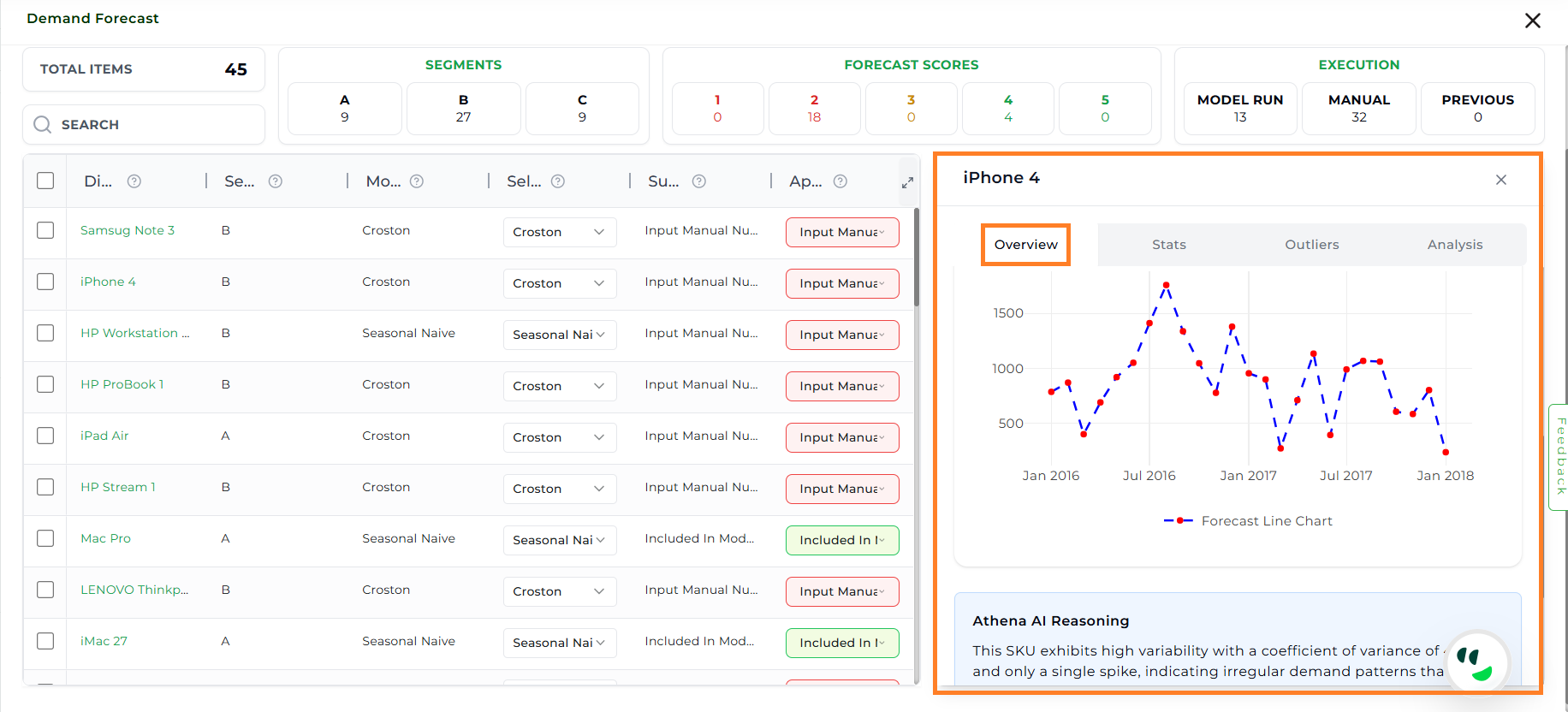
Overview#
The Overview section provides key forecastability measures, visualizations, and reasoning from Athena AI.
Metrics
Athena Forecast Score
Coefficient of Variance: A percentage-based measure of variability, helping spot volatile vs. stable items.
ADI (Intermittency): Measures the sparsity of demand. It answers the question: “How often does this item sell?” A low ADI means the item sells frequently and consistently.
Trend Strength: Measures the direction of demand over time. It answers the question: “Is there a consistent, long-term growth or decline in sales?”
Seasonality Strength: Measures the cyclicality of demand. It answers the question: “Does demand have predictable peaks and troughs that repeat over a set period?”
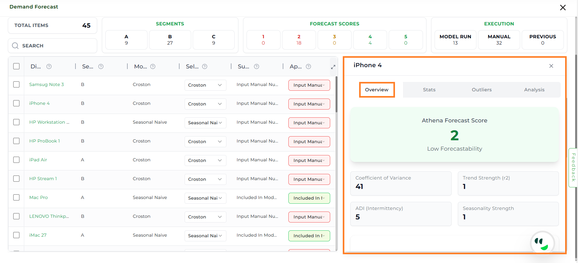
Overview#
Forecast Visualization
Forecast Line Chart: A historical line plot that displays the progression of data points over time, showing how values have changed across a historical period. It helps in visualizing trends, patterns, and shifts in the data, making it easier to compare past behaviors and understand long-term movements.
Athena AI Reasoning
Provides an explanation of why a particular model is best suited by analyzing the statistical properties of the historical data.
Considers factors such as variability, seasonality, trend, and patterns in the dataset to justify the model selection.
This reasoning provides transparency into the decision-making process, helping users understand how data characteristics influence model suitability.
Overview#
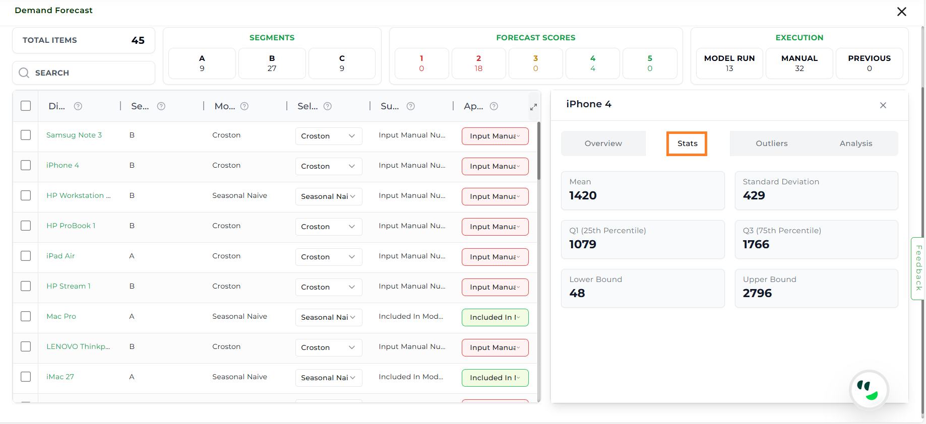
Statistics (Stats)#
The Stats section provides descriptive statistical measures of the forecast.
Mean: Gives the average expected demand over the forecast period.
Standard Deviation: Measures how spread out the forecast values are, which affects planning confidence.
First Quartile (Q1): Shows the lower end of typical demand range, useful for identifying underperforming periods.
Third Quartile (Q3): Shows the higher end of typical demand range, useful for identifying peak performance.
Lower Bound: Sets the minimum acceptable range for forecast data; values below this may be anomalies.
Upper Bound: Sets the maximum acceptable range for forecast data; values above this may be anomalies.
Statistics#
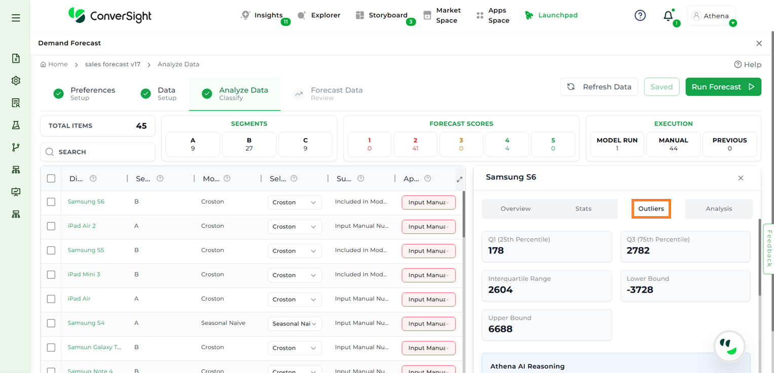
Outliers#
The Outliers section highlights deviations from expected demand patterns.
Metrics
Detection Method: The statistical technique used to identify outliers in the dataset.
Imputation Method: The approach applied to replace or estimate missing or anomalous values.
Detection Level: The level at which outlier detection is performed, such as item-level or aggregated level.
Multiplier: The factor multiplied with the IQR to define the acceptable data range for outlier detection.
Q1 (25th Percentile): Represents the value below which 25% of the data points fall.
Q3 (75th Percentile): Represents the value below which 75% of the data points fall.
Interquartile Range (IQR): The difference between Q3 and Q1, showing the middle 50% spread of the data.
Lower Bound: The minimum threshold calculated to detect values that fall significantly below the normal range.
Upper Bound: The maximum threshold calculated to detect values that fall significantly above the normal range.
Number of Outlier Instances: The count of data points identified as outliers based on the defined thresholds.
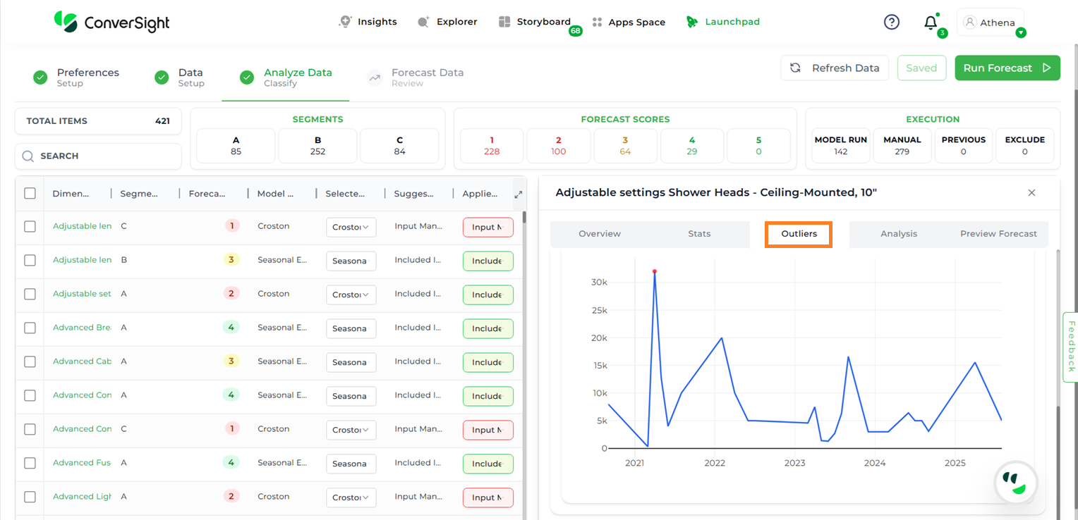
Visualization
Outlier Line Plot: Highlights data points in a time series that deviate significantly from the expected pattern. The underlying line shows the original data, while outliers are distinctly marked to make anomalies easy to spot. This visualization helps in quickly identifying unusual spikes, drops, or irregular behavior in the series.
Outlier#
Outlier#
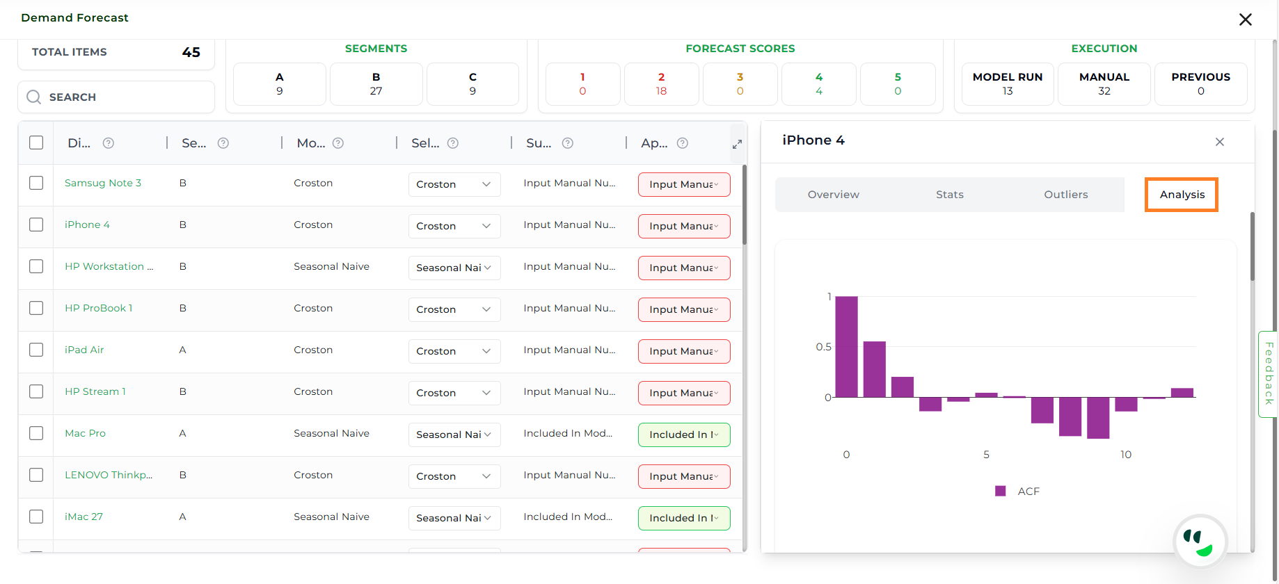
Analysis#
The Analysis section provides advanced diagnostic graphs to understand demand behavior.
Autocorrelation Function (ACF) Plot: Shows the correlation between a time series and its past values across different lags. Useful for identifying repeating patterns, seasonality, and how strongly current values depend on previous observations.
Partial Autocorrelation Function (PACF) Plot: Displays the direct correlation between a time series and its lagged values after accounting for shorter lags. Highlights the independent influence of each lag.
Seasonal Decomposition of Time Series (SDL) Plot: Separates the series into trend, seasonality, and residual components.
Trend: Captures long-term movement.
Seasonality: Reflects repeating short-term cycles.
Residuals: Shows random variation not explained by the other components.
Observed Graph: Displays raw historical demand.
Trend Graph: Shows long-term upward or downward movements.
Seasonal Graph: Captures repeating demand cycles.
Residual Graph: Highlights random noise or unexplained variability.
Analysis#
Preview Forecast#
Users can generate a forecast for a specific item to view the corresponding graphs across multiple models—without needing to run the entire forecast each time for individual items or different model configurations.
After selecting the desired item, click on the Preview Forecast tab. A list of all available models will appear.
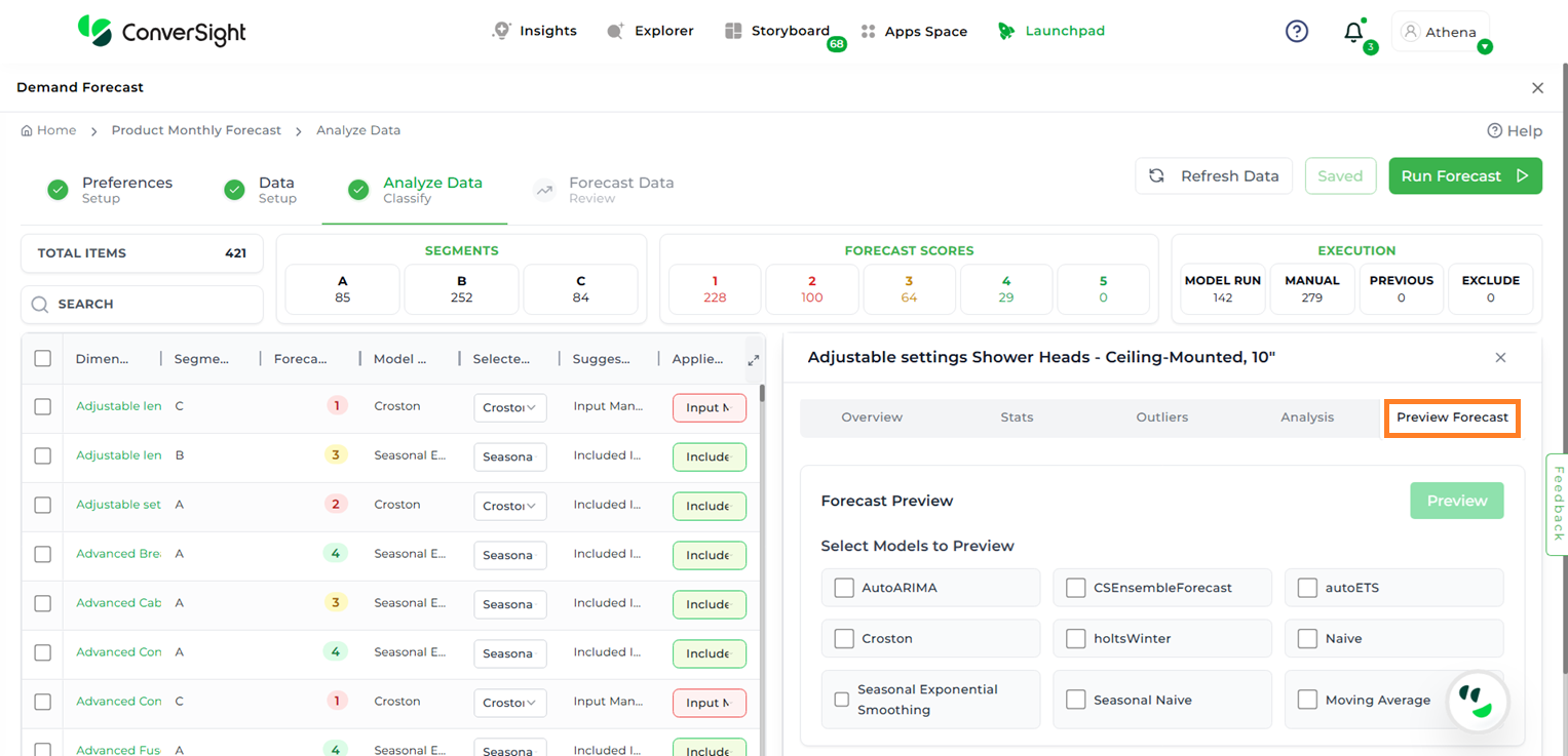
Preview Forecast#
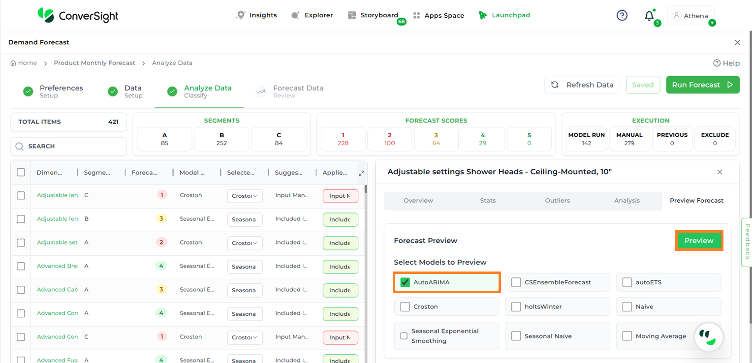
Choose the required model and click Preview to view the forecast results.
Forecast Model Preview#
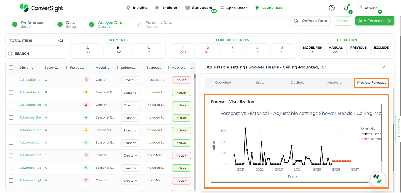
Forecast Model Preview#
Forecast Inclusion / Exclusion Rules#
The Demand Forecast app automatically evaluates each item or segment against a set of predefined conditions to decide whether it should be included in, excluded from, or carried over in the forecast. These rules are applied dynamically during each analysis run, based on the latest data and configured thresholds.
Inclusion Criteria#
An item or segment is included in the forecast when it does not meet any exclusion conditions. In such cases, the action field is marked as Included.
Exclusion Criteria#
An item or segment is excluded from the forecast when it meets any of the following conditions:
Outlier Instances greater than or equal to seven Represents the number of periods in which the product’s demand deviates significantly from the expected range. A threshold of seven is applied to filter out products with excessive and unpredictable demand variations.
Zero Instances greater than or equal to six Represents the number of periods in which the product recorded zero sales or demand. A threshold of six indicates that the product is considered inactive if it has recorded zero demand for at least five periods in the observed timeframe.
Negative Instances greater than or equal to six Represents the number of periods with negative sales values, often caused by returns or adjustments. A threshold of six is applied to prevent erroneous forecasting for products with excessive returns.
Frequency less than six Represents how often a product was purchased or ordered within the observed timeframe. A value below six indicates irregular demand, making the product less reliable for forecasting.
Recency greater than or equal to five Represents the number of periods since the product was last sold. A value of five or more indicates low recent demand, suggesting the product is outdated for forecasting purposes.
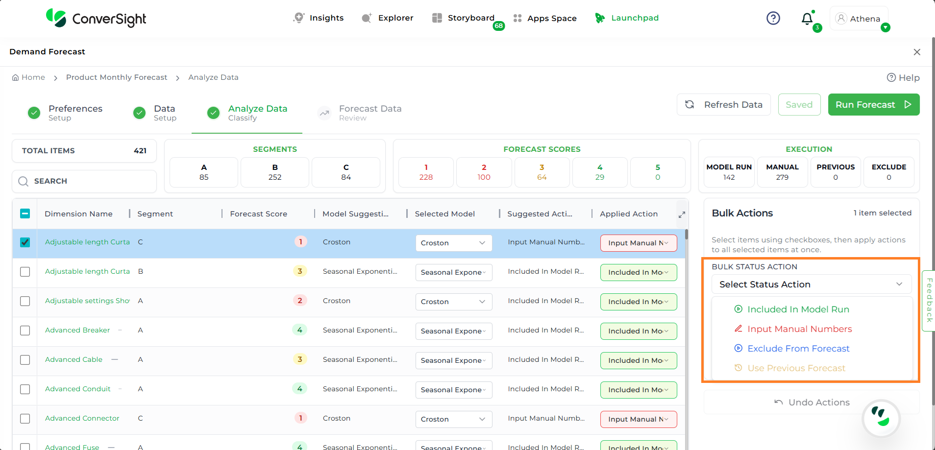
Bulk Actions#
The Bulk Actions feature enables users to apply forecast-related actions to multiple dimension values at once, streamlining the data preparation process. This feature becomes visible only when a dimension name or multiple dimension names are selected.
There are three main options available under Bulk Actions:
Bulk Status Action
Selected Model
Substitute Items
Bulk Status Action
This option enables users to apply specific status updates to the selected data using a dropdown menu. The available choices include:
Include in Model Run – Marks the selected items to be included in the forecasting model.
Input Manual Numbers – Allows users to manually input forecast values for the selected items.
Exclude from Forecast – Excludes the selected items from the forecast.
Use Previous Forecast – Applies values from a prior forecast to the selected items.
Bulk Status Action#
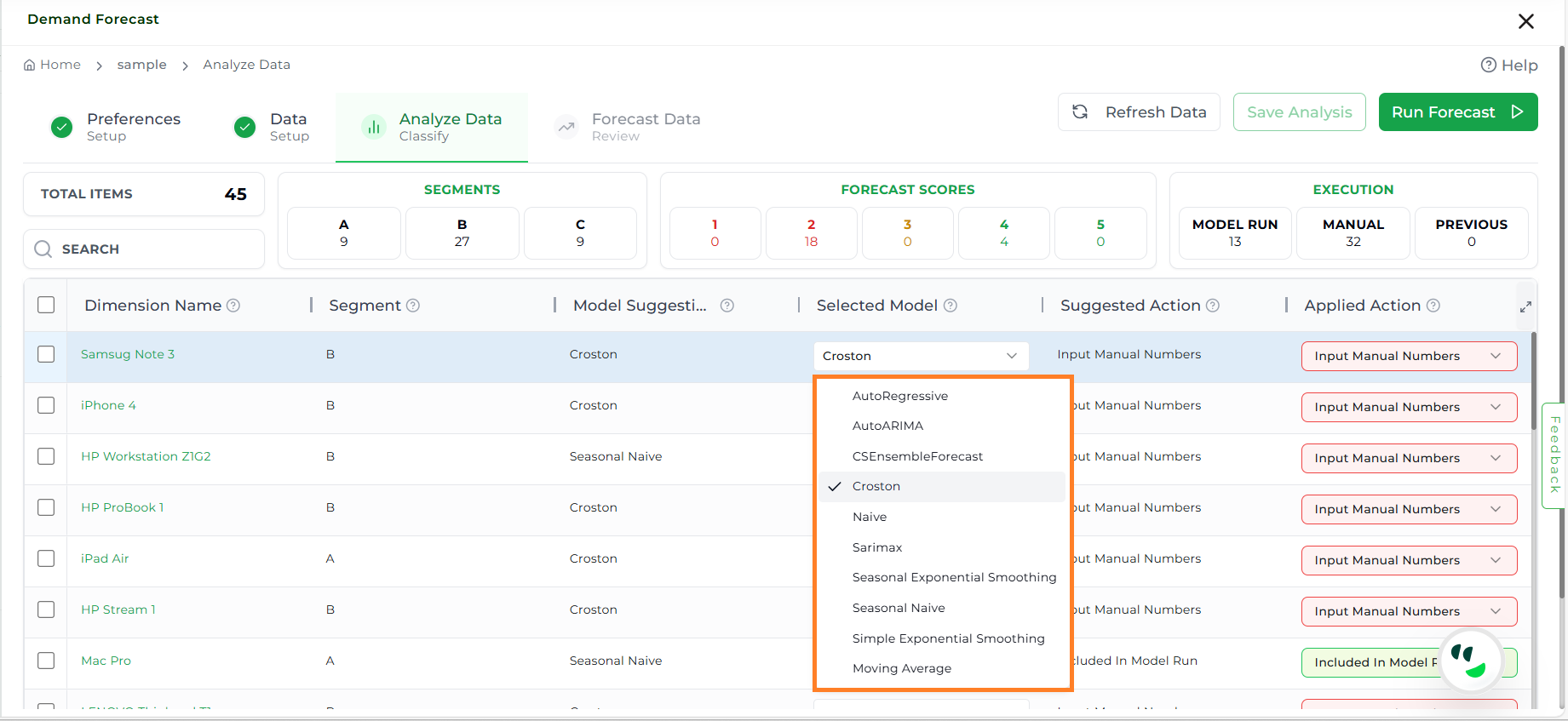
Selected Model
The Selected Model option enables users to modify the forecasting model currently in use, either to align with their preferences or to generate forecasts using a different model. Users can choose their desired forecasting model from the available dropdown list.
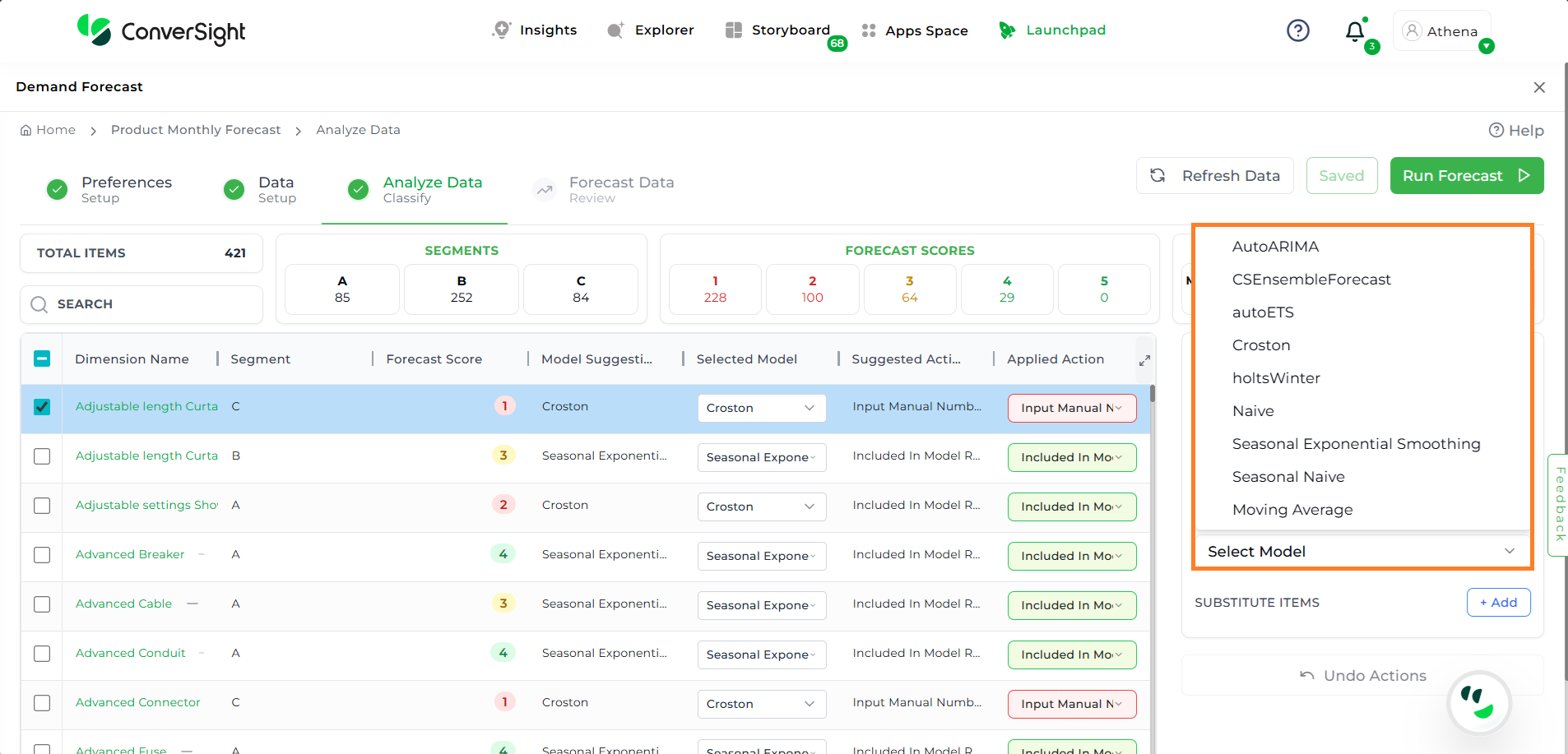
Selected Model#
Substitute Items
The Substitute Items option allows users to assign one or more alternate (substitute) items for an existing item used in the forecast. Users can apply substitute item values to the forecast using either the Simple Average, Weighted Average or the Sum method.
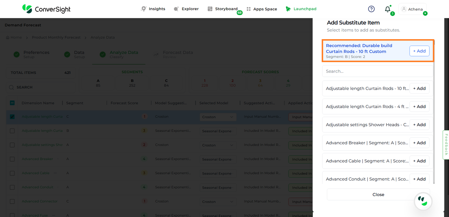
To add substitute items, click the Add button. A list of eligible items will appear.
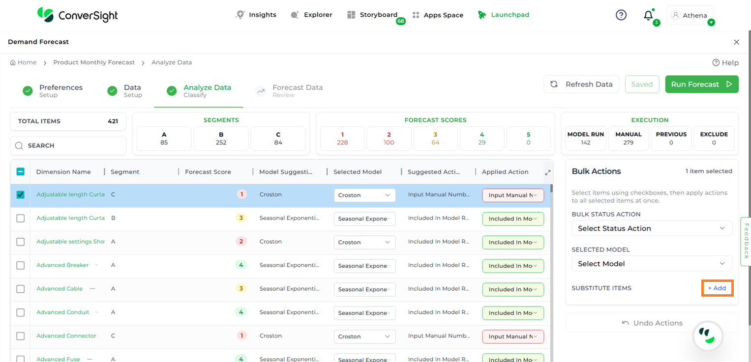
Substitute Items#
Users can then click the Add button next to the desired item(s) to include them as substitutes. By default, the app provides a recommendation for which item is more suitable to be substituted.
NOTE
A recommendation will be provided only when a single dimension is selected. No recommendation will be generated if multiple dimensions are selected.
Substitute Items#
Once a substitute item is added, it will appear in the Bulk Actions section under the Substitute Items option. Users can also apply a scaling factor and weight to the added item, adjusting it as needed to align with specific business requirements.
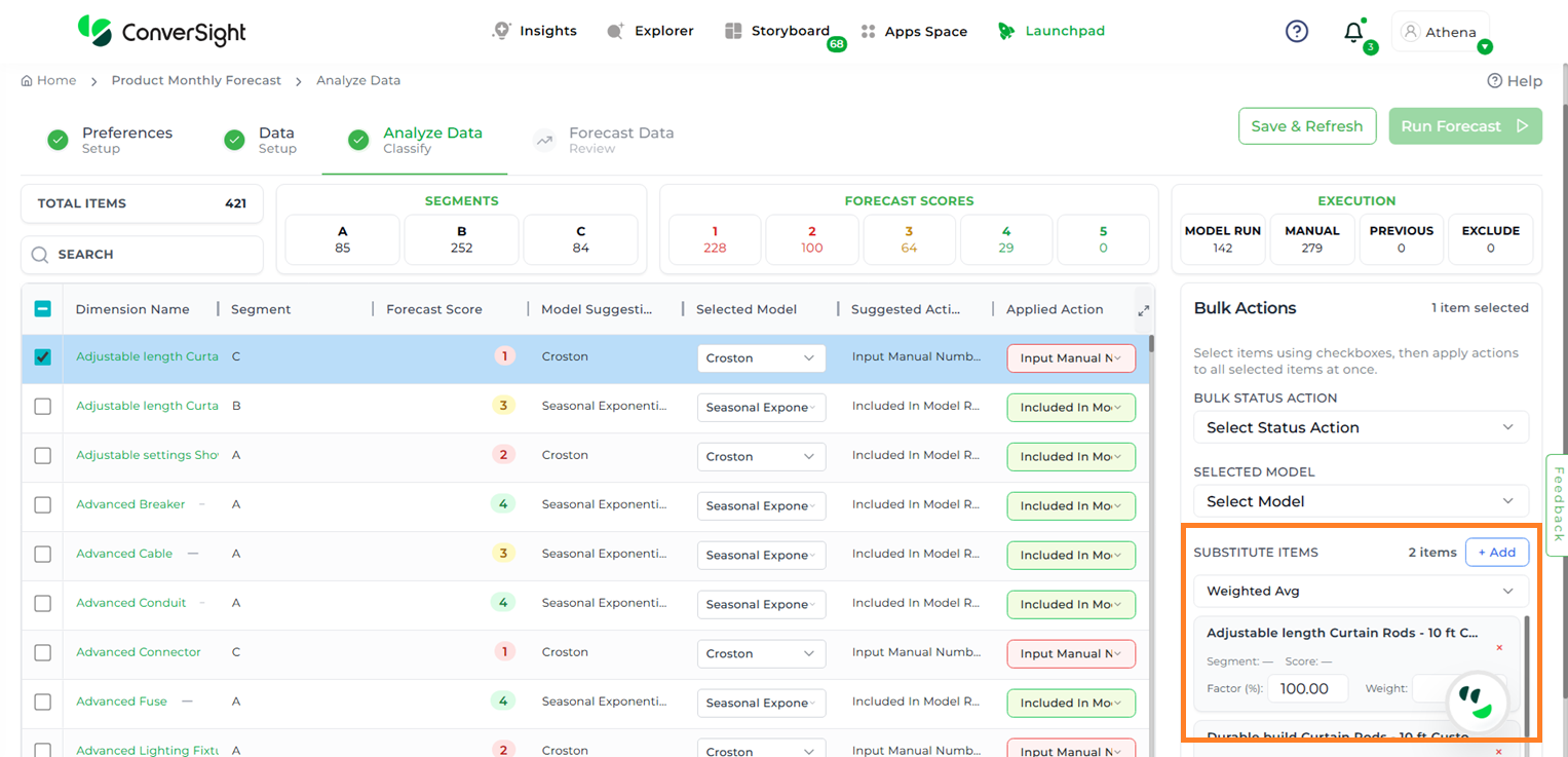
Substitute Items#
NOTE
The Use Previous Forecast option is disabled for scenarios that are being created for the first time, as no historical forecast data is available.
If any changes need to be reverted, the Undo Actions button allows users to undo all applied bulk actions instantly.
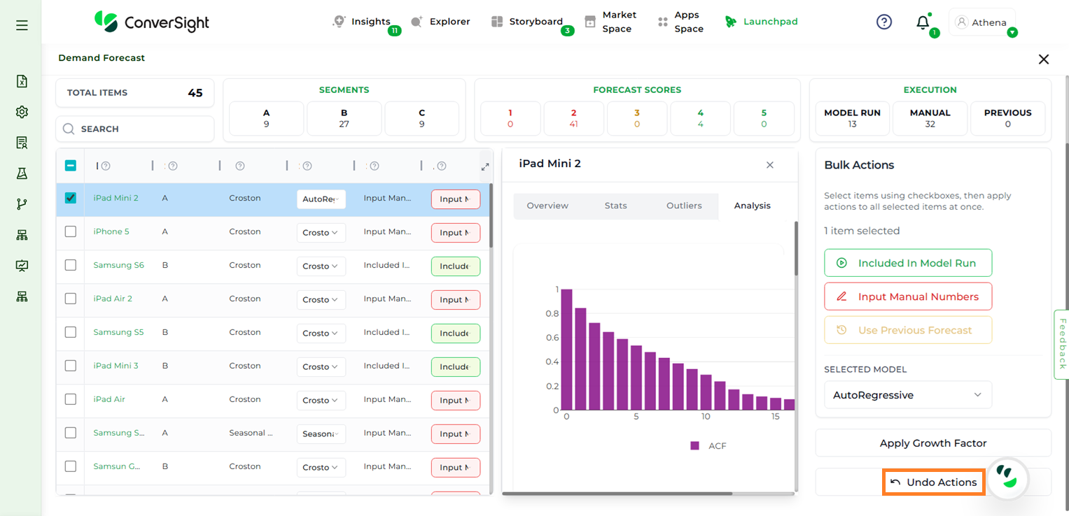
Undo Actions#
NOTE
To run the forecast, the Applied Action must be set to Included in Model Run for at least two SKUs.
After making the necessary changes during the analysis process, users can click the Save Analysis button to save their progress. This ensures that all modifications made to the data and applied actions are retained.
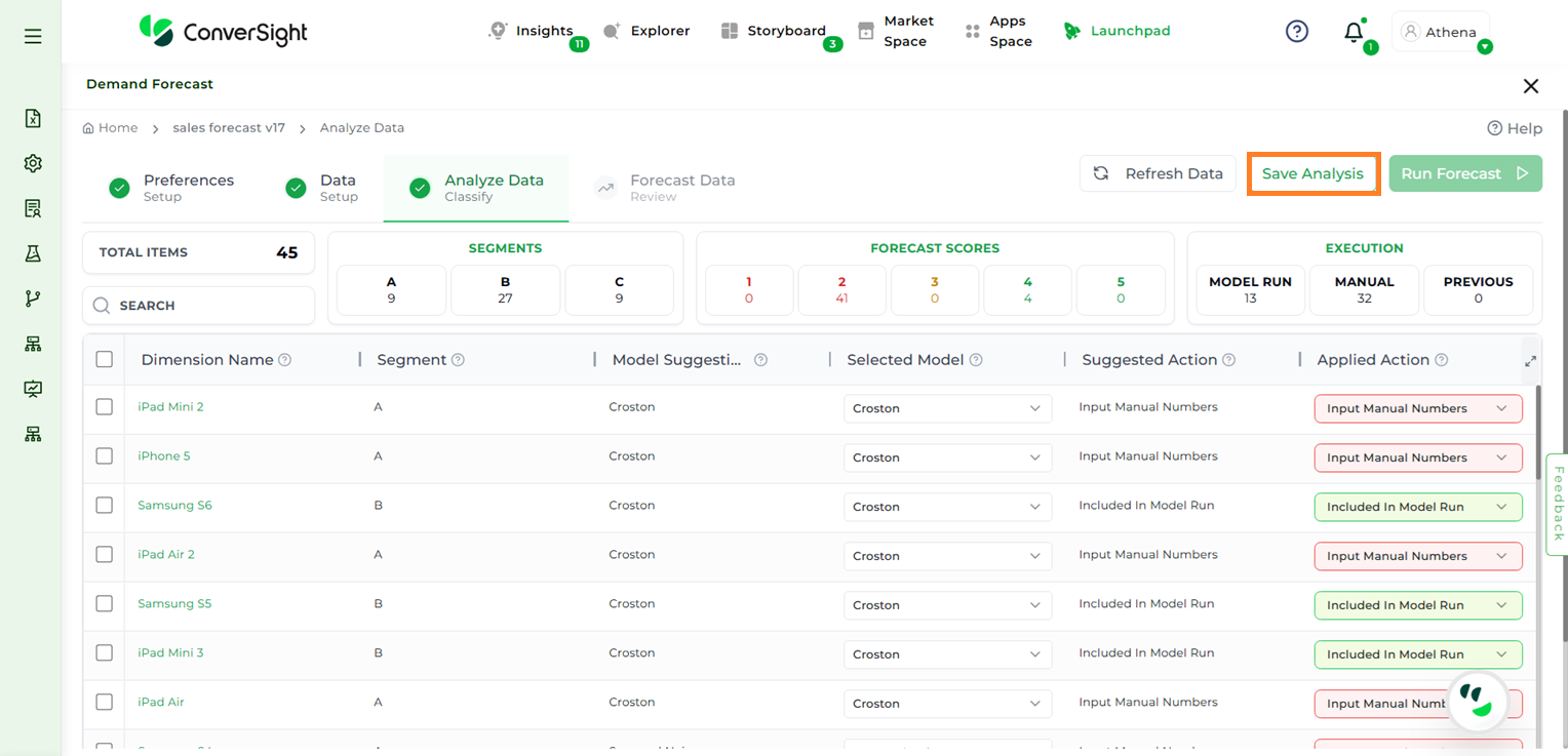
Save Analysis#
Once the analysis is saved, click on the Run Forecast button to initiate the forecasting process based on the current data setup and applied actions.
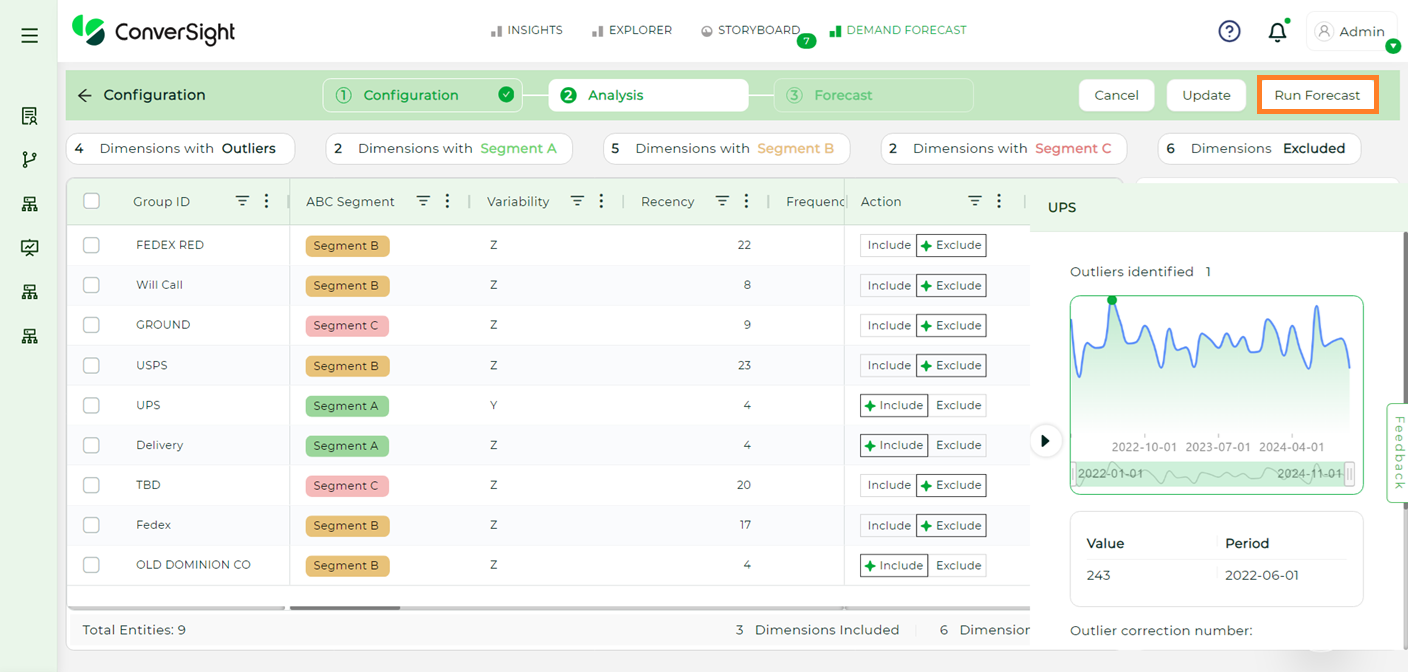
Run Forecast#
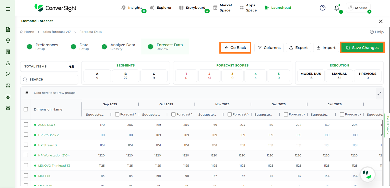
Forecast Data#
The Forecast Data page presents forecasted values in a detailed table format, enabling users to review projections at a granular level. Users can utilize the Search bar to locate specific dimension columns quickly and efficiently.
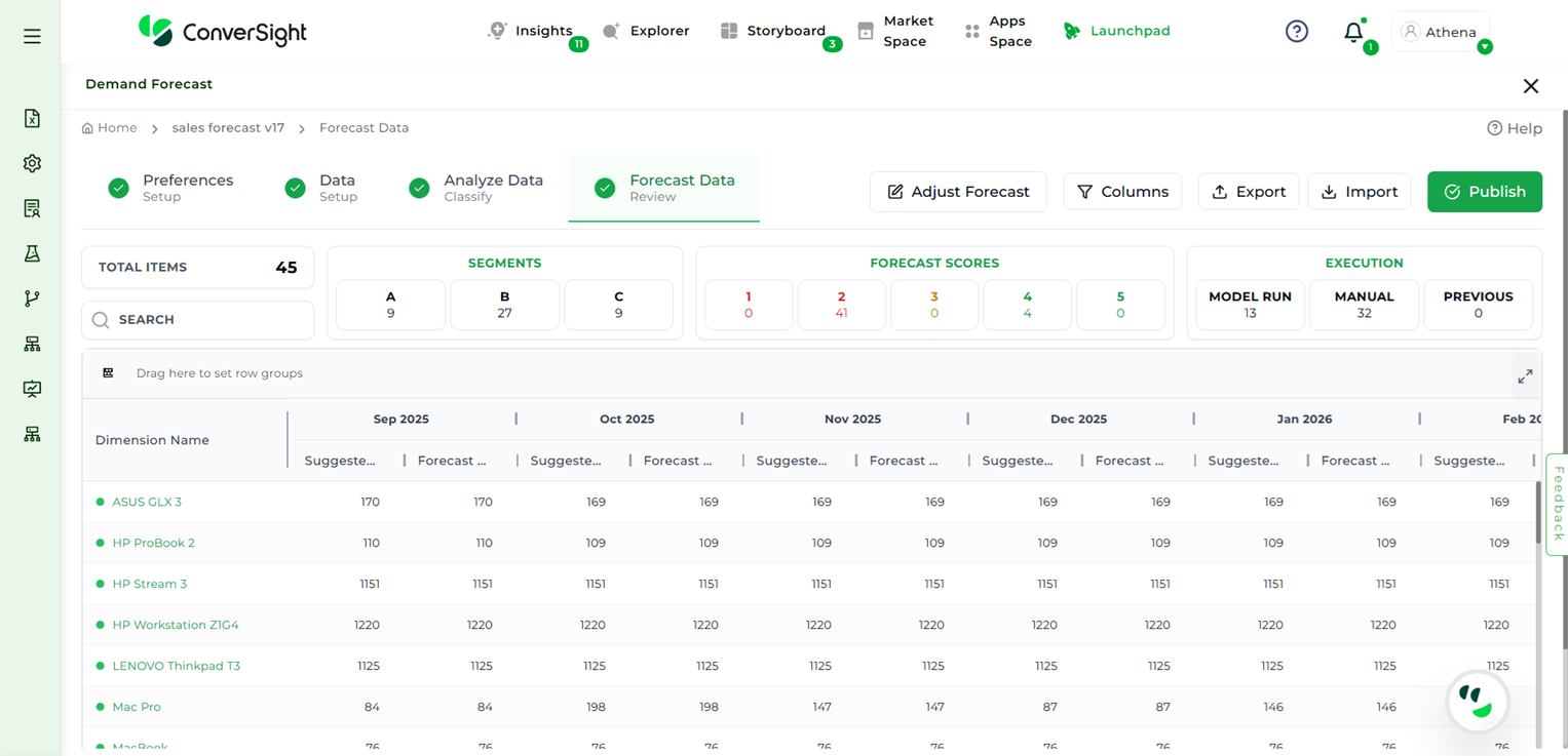
Forecast Page#
Adjust Forecast#
To make changes to forecasted values, users can click the Adjust Forecast button. This functionality allows for manual modifications tailored to specific business requirements.
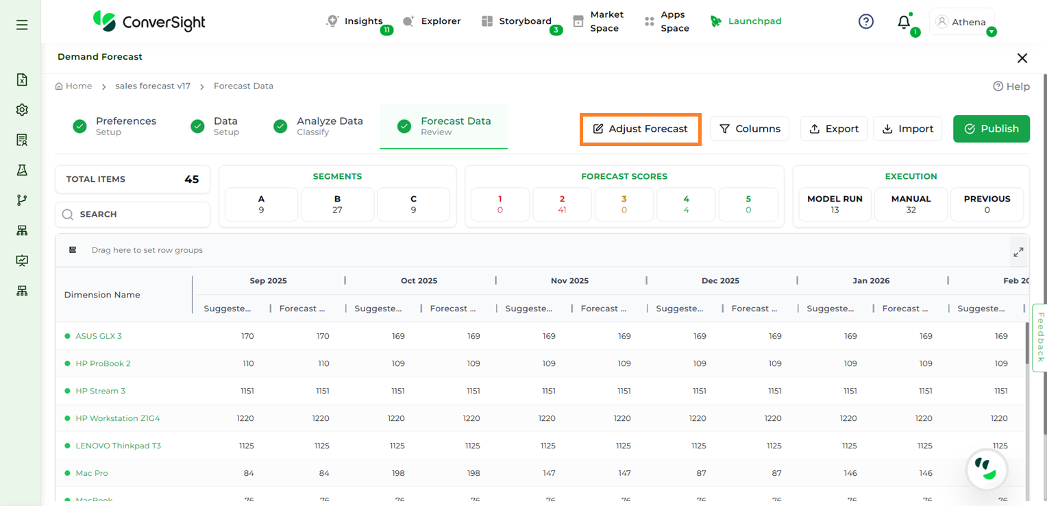
Adjust Forecast#
The forecast table includes the following
Column Name |
Description |
|---|---|
Dimension Name |
This is the name of the item or segment being forecasted. |
Date |
This represents the period associated with each forecast entry. |
Prior Approved |
Displays the forecast value that was approved or published earlier for the specified item and period. |
Suggested |
Represents the values currently recommended by the forecasting model for the specified dimension and date. |
Change |
Displays the difference between the model’s suggested value and the previously approved forecast. |
Actual Value |
The true historical values observed for that period and dimension. |
Forecast |
The final forecast value for this entry. This column is editable, allowing users to review or override model suggestions before publishing. |
Upon clicking Adjust Forecast, users can select any cell in the table to enter updated values. When a cell is selected, a Growth Factor section also appears, allowing users to apply growth factors directly to the forecasted data.
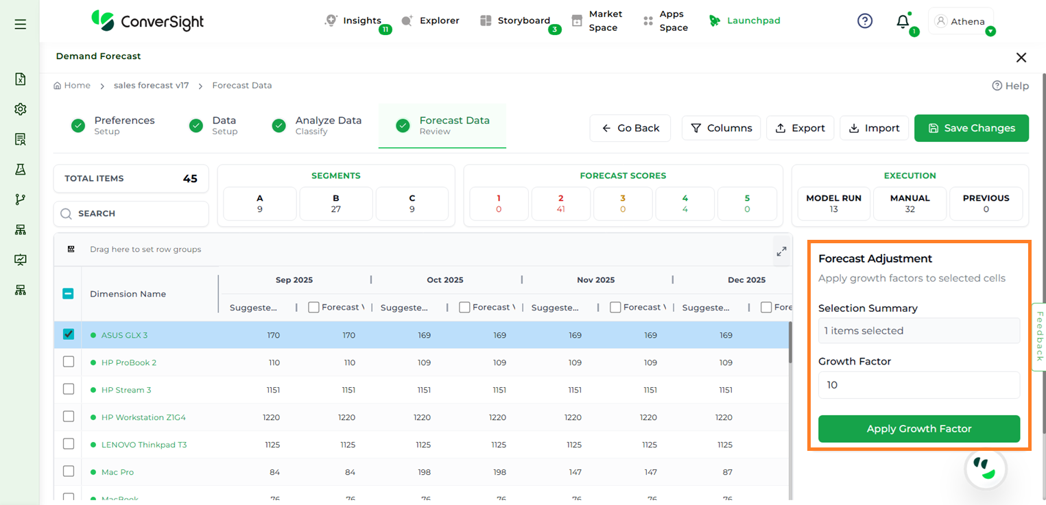
Forecast Adjustment#
Once the adjustments are complete, click Save Changes to apply and retain the modifications.
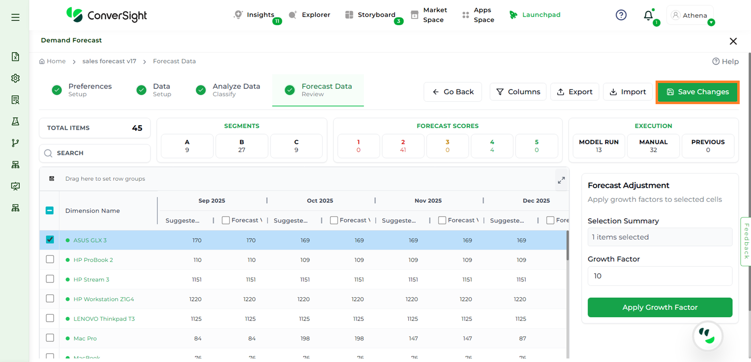
Save Changes#
NOTE
All manual inputs and adjustments made to the forecast will persist and carry over when using the Use Previous Forecast option. This streamlines the forecasting process by eliminating the need to recreate forecasts from scratch.
Columns#
Users can customize the table view using three options: Forecast Values, Forecast Volume, and System Columns. To apply these filters, click the Columns button and choose the desired options from the dropdown.
Forecast Values: Displays the forecasted unit value of an item or segment when enabled.
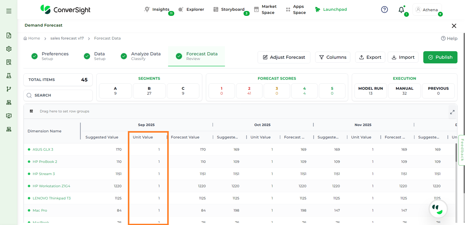
Forecast Values#
Forecast Volume: Displays the forecasted volume of an item or segment when enabled.
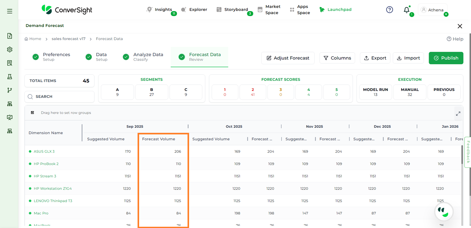
Forecast Volume#
System Columns: Displays system details such as forecast creation date, creator, last updated date, last updated by, and the forecast period when enabled.
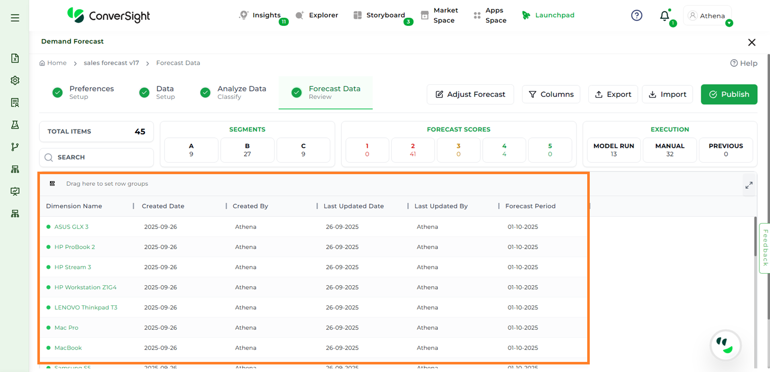
Forecast Volume#
Export#
Click the Export button to export the forecasted data in CSV format. This allows for offline review or further analysis.

Export#
Import#
Users can upload a CSV file using the Import CSV button. This is useful for two scenarios:
Uploading a custom CSV file to run the forecast
Making changes to the downloaded CSV file and re-uploading the updated version
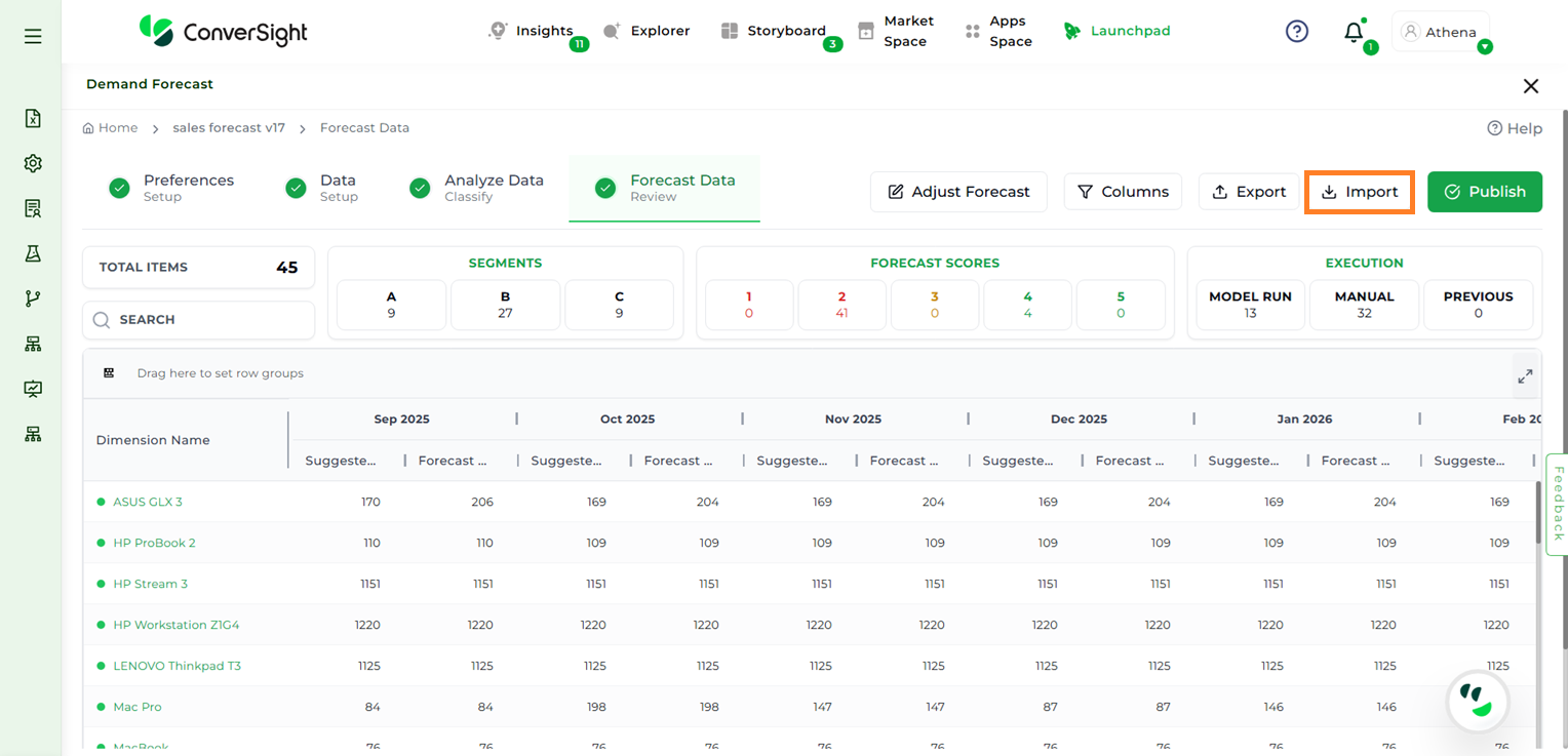
Import#
After adjusting values manually or importing the updated CSV, users must click Save Changes to apply the updates and then click the Go Back button if no further changes need to be done.
Demand Forecast#
NOTE
The download and import CSV functionality are available exclusively for manual forecasted values. You cannot overwrite model-generated (automated) predictions directly using this feature—only those values marked for manual forecasting can be updated in this way.
Publish#
The Publish button allows users to make the created forecast accessible across the organization. Once published, all users can view and edit the forecast as required.
Users can publish a forecast in three ways:
Create New Forecast – Generates a completely new forecast. When this option is selected, users will be prompted to enter a name for the new forecast.
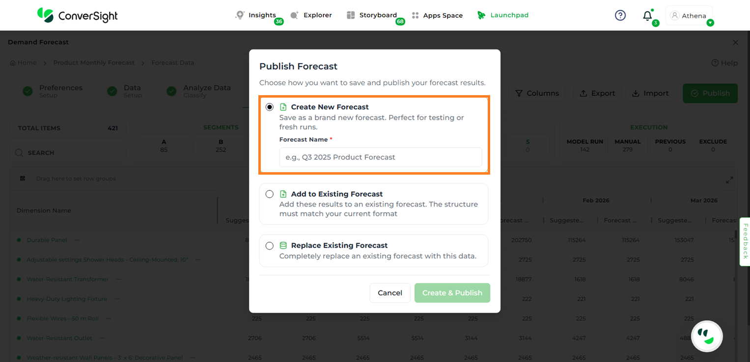
Publish by Creating New Forecast#
Add to Existing Forecast – Appends the results of the current forecast to an existing one. Users must select the target forecast from the dropdown list.
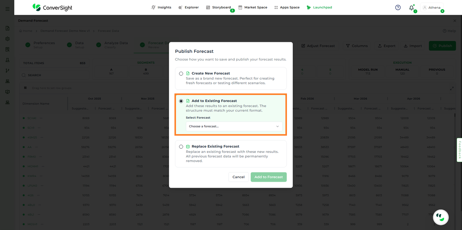
Publish by Adding to Existing Forecast#
In this step, schema validation is performed. If a schema mismatch is detected, the system will indicate whether any columns are missing or additional.
There are two ways to resolve this issue: using the Update + Insert method or the Insert method.
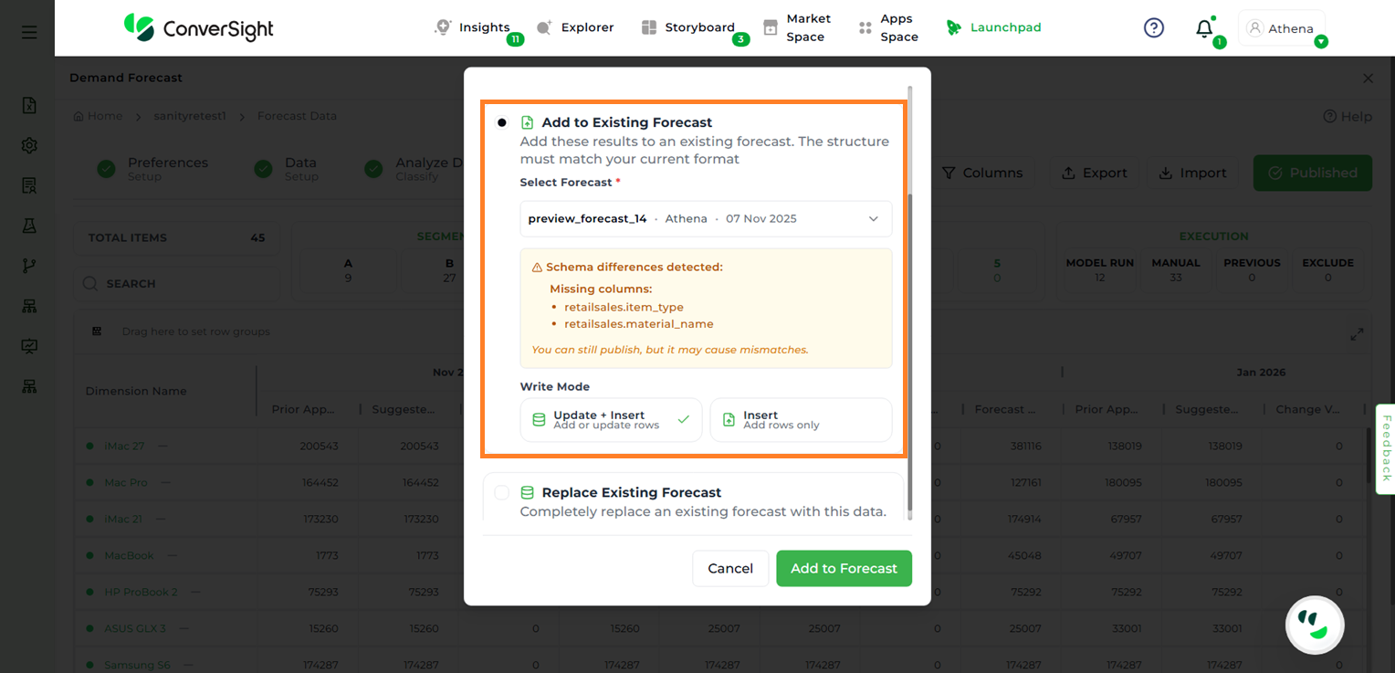
Schema Mismatch#
Replace Existing Forecast – Replaces an existing forecast entirely with the new results. All previously stored forecast data will be permanently deleted.
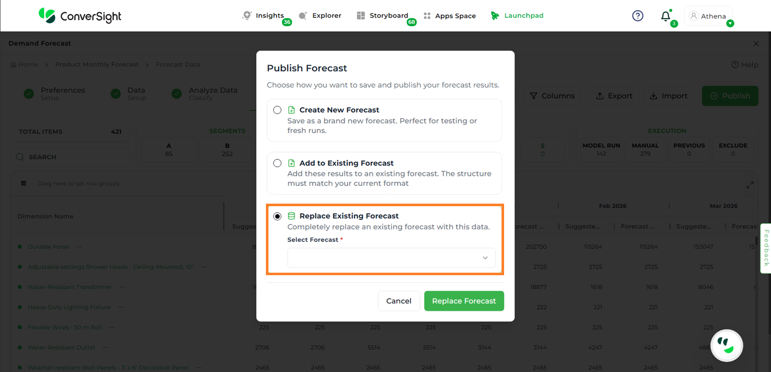
Publish by Replacing Existing Forecast#